Sklearn 线性回归：完整指南与示例

线性回归是统计学和机器学习中的基础技术，用于建模变量之间的关系。简单来说，它可以根据一个或多个影响因素来预测结果。它广泛应用于房产定价、销量预测、风险评估等诸多领域。

在本教程中，我们将探索 scikit-learn 中的线性回归，涵盖其工作原理、适用原因，以及如何用 scikit-learn 实现。读完后，您将能够构建并评估线性回归模型，以进行数据驱动的预测。

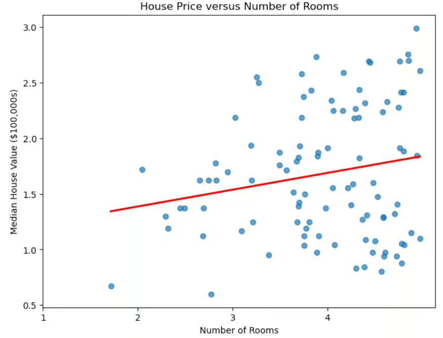
房价与房间数量的散点图

线性回归与机器学习

除了用于估算房价的直接用途外，线性回归在机器学习中也扮演着重要角色。

• 它是理解更高级技术（如 逻辑回归、神经网络 和 支持向量机）的基石。
• 训练速度快，适合快速原型开发。
• 它还能作为对比的基线模型。如果更复杂的模型并未显著优于它，额外的复杂度未必值得。
• 不同于某些技术（如深度学习），它易于解释。
• 它可以辅助特征选择，识别最有用的预测因子。

尽管简单，线性回归因其高效、可解释和通用性，仍是机器学习中不可或缺的工具。

线性回归与 scikit-learn 库

scikit-learn 让线性回归的实现变得容易。该库具有许多优势。

• 接口一致。实现不同机器学习算法所需的代码风格相似。
• 代码简洁，复杂的数学与实现细节被抽象化。例如在训练集上拟合模型，只需一行 model.fit(X_train, y_train)。
• 可轻松访问模型系数。
• 内置评估模型性能的指标。
• 借助 Pipeline，线性回归（或任何其他算法）与预处理步骤（如缩放、特征选择）易于集成。

如果您是 scikit-learn 新手，可以查看我们的课程 使用 scikit-learn 的机器学习，获得对此 Python 库的动手入门。 

理解线性回归

如前所述，在简单线性回归中，数据用一条“最佳拟合直线”来建模。其公式为： 

其中 m 为斜率，b 为截距。

“多元线性回归”将单一自变量的情形推广到多个自变量（房间数量、是否临海、社区的收入中位数）。其公式推广为： 

其中每个 x_i 是自变量，对应的 b_i 是其系数。在三维空间中，直线推广为平面；在更高维中，平面变为“超平面”。

如何解释系数和截距？截距是在所有自变量为 0 时对 y 的预测值，换言之，是在预测因子不贡献时因变量的基线值。每个系数 b_i 表示当 x_i 变化一个单位、且其他自变量保持不变时，因变量 y 的变化量。

环境配置

安装 scikit-learn 很简单。直接使用命令 pip install scikit-learn 即可。若需安装特定版本（如 1.2.2），可在命令中指定版本： pip install scikit-learn==1.2.2. 如果您使用 Anaconda，scikit-learn 通常已预装。若在 Anaconda 发行版中仍需安装，请使用 conda install scikit-learn。

在使用 scikit-learn 时，有几类库是必要或推荐的。 numpy 用于存储特征与标签；pandas 推荐用于加载、预处理与探索数据集。 

如果您在用 scikit-learn，很可能已用 pandas 做数据准备。要绘图，通常会使用 matplotlib 或 seaborn，或两者兼用。以上库均可用 pip 安装，和前述示例类似。甚至可以用一条命令一次安装多个库：

pip install scikit-learn numpy pandas matplotlib seaborn。

在 sklearn 中实现线性回归

在加载数据集之前，先导入常用库。

# Import libraries.
import numpy as np
import pandas as pd
import matplotlib.pyplot as plt
import seaborn as sns

加载数据集

我们使用著名的加州房价数据集。

# Read in California housing dataset.
from sklearn.datasets import fetch_california_housing


housing = fetch_california_housing()

准备数据

我们将数据拆分为训练集与测试集。先从 sklearn.model_selection 导入 train_test_split()，再调用它，指定测试集比例与 random_state。我们还将使用简单线性回归，选择平均房间数这一特征。

# Import train_test_split.
from sklearn.model_selection import train_test_split


# Create features X and target y.
X = pd.DataFrame(housing.data, columns=housing.feature_names)[["AveRooms"]]
y = housing.target  # Median house value in $100,000s


# Split the dataset into training (80%) and testing (20%) sets.
X_train, X_test, y_train, y_test = train_test_split(X, y, test_size=0.2, random_state=42)

完成训练集与测试集的划分后，我们对特征进行标准化。这可使各变量处于相同量纲，从而提升模型性能与数值稳定性。

# Import StandardScaler.
from sklearn.preprocessing import StandardScaler

# Instantiate StandardScaler.
scaler = StandardScaler()

# Fit and transform training data.
X_train_scaled = scaler.fit_transform(X_train)

# Also transform test data.
X_test_scaled = scaler.transform(X_test)

在这段代码中，StandardScaler 是一种预处理工具，用于去均值并将特征缩放到单位方差。这有助于避免因量纲差异导致某些特征主导模型。

通过 fit_transform() 在训练数据上拟合并变换。随后使用 transform() 单独变换测试数据，以确保使用与训练数据相同的缩放系数，避免数据泄漏。

训练线性回归模型

要创建线性回归模型，从 sklearn.linear_model 导入 LinearRegression()，实例化并赋给变量。

# Import LinearRegression.
from sklearn.linear_model import LinearRegression


# Instantiate linear regression model.
model = LinearRegression()

用训练数据拟合模型非常直接。

# Fit the model to the training data.
model.fit(X_train_scaled, y_train)

进行预测

完成模型训练后，我们在测试集上进行预测。

# Make predictions on the testing data.
y_pred = model.predict(X_test_scaled)

评估模型性能

在得到测试集的预测结果后，需要了解其与真实情况的匹配程度。评估回归算法性能有多种指标，常见的包括判定系数（R²）、均方误差（MSE）和均方根误差（RMSE）。

判定系数 R² 用于衡量回归模型对目标变量变异性的解释程度。换言之，它量化了预测因子对目标变量的解释比例，即“拟合优度”。

为进一步理解，来看其公式：

其中 yactual 为目标变量真实值，ypredicted 为模型预测值，ȳ 为真实值的均值。该公式帮助我们理解模型解释目标变量方差的程度。分母表示数据的总方差，分子表示应用回归模型后未被解释的方差。两者比值即为模型解释的方差百分比。

如何解读 R²？

• R² = 1：模型完美解释了目标变量的全部方差。 
• R² = 0：模型未解释任何方差；预测不优于直接使用均值。 
• R² < 0：模型甚至劣于使用均值，表明拟合很差。

需要注意的几点：

• 更高的 R² 并不总是更好。过高的 R² 可能表示过拟合，尤其在复杂模型中。 
• 增加更多特征会人为提高 R²，因此更高的数值未必更优。
• 对多元回归，应使用调整后的 R²，其考虑了预测因子数量，可避免无关变量带来的误导性提升。

在 scikit-learn 中使用判定系数评估模型性能非常方便。

# Import metrics.
from sklearn.metrics import mean_squared_error, r2_score


# Calculate and print R^2 score.
r2 = r2_score(y_test, y_pred)
print(f"R-squared: {r2:.4f}")

R-squared: 0.0138

其他常用指标包括均方误差（MSE）和均方根误差（RMSE）。它们衡量模型预测与真实值之间的偏差程度。

MSE 计算真实值与预测值之差的平方的平均值： 

其中 n 为观测总数。由于在平均前对误差进行了平方，较大的误差会受到更重的惩罚，因此 MSE 对离群点较敏感。MSE 越低，模型拟合越好。

为缓解该问题，可使用 RMSE，即 MSE 的平方根。由于 RMSE 与目标变量具有相同单位，更便于解释平均预测误差的大小。

使用 scikit-learn 计算 MSE 与 RMSE 十分容易。

# Calculate and print MSE.
mse = mean_squared_error(y_test, y_pred)
print(f"Mean squared error: {mse:.4f}")


# Calculate and print RMSE.
rmse = mse ** 0.5
print(f"Root mean squared error: {rmse:.4f}")

Mean squared error: 1.2923
Root mean squared error: 1.1368

在 scikit-learn 中使用多元线性回归

我们使用所有可用特征重新运行模型，而不仅是平均房间数。您认为结果会更好还是更差？

# Uses all features.
import numpy as np
import pandas as pd
import matplotlib.pyplot as plt
import seaborn as sns
from sklearn.datasets import fetch_california_housing
from sklearn.model_selection import train_test_split
from sklearn.preprocessing import StandardScaler
from sklearn.linear_model import LinearRegression
from sklearn.metrics import mean_squared_error, r2_score


# Load data set.
housing = fetch_california_housing()


# Split into X, y.
X = pd.DataFrame(housing.data, columns=housing.feature_names)
y = housing.target  # Median house value in $100,000s
X_train, X_test, y_train, y_test = train_test_split(X, y, test_size=0.2, random_state=42)


# Scale the data.
scaler = StandardScaler()


X_train_scaled = scaler.fit_transform(X_train)
X_test_scaled = scaler.transform(X_test)


# Create model and fit it to the training data.
model = LinearRegression()
model.fit(X_train_scaled, y_train)


# Make predictions.
y_pred = model.predict(X_test_scaled)


# Calculate and print errors.
r2 = r2_score(y_test, y_pred)
print(f"R-squared: {r2:.4f}")


mse = mean_squared_error(y_test, y_pred)
print(f"Mean squared error: {mse:.4f}")


rmse = mse ** 0.5
print(f"Root mean squared error: {rmse:.4f}")

R-squared: 0.5758
Mean squared error: 0.5559
Root mean squared error: 0.7456

可以看到，结果明显优于仅使用一个特征的情况。不过，这也引出了是否需要所有特征的问题：有些特征是否更为相关？从数据集中选择最相关的特征称为特征选择。

特征选择之所以重要，原因有：

• 减少过拟合。更少的特征意味着更低的复杂度，从而降低过拟合风险。
• 提升准确性。移除无关或冗余特征可使模型聚焦于有意义的模式。
• 增强可解释性。突出最重要因素，让模型更易理解。
• 加快训练。减少特征数量可降低计算时间与内存占用。

当多个特征高度相关时，它们是冗余的，即向模型提供了本质相同的信息。这种情况称为多重共线性。虽然多重共线性不一定影响预测模型的精度，但会使特征选择和解释变得复杂，尤其在线性回归及相关模型中。

方差膨胀因子（VIF）是用于检测自变量间多重共线性的度量。对每个自变量，VIF 的计算为： 

其中 R_i² 是将预测因子 X_i 对其他所有预测因子回归得到的 R²。VIF 越高，表示该预测因子与其他变量的相关性越强。

• VIF = 1：无多重共线性（理想）。
• VIF < 5：低到中度多重共线性（通常可接受）。
• VIF > 5：高度多重共线性（考虑移除或合并相关变量）。
• VIF > 10：严重多重共线性（强烈暗示变量冗余）。

# Import libraries.
import numpy as np
import pandas as pd
import seaborn as sns
import matplotlib.pyplot as plt
from sklearn.datasets import fetch_california_housing
from statsmodels.stats.outliers_influence import variance_inflation_factor


# Load the dataset.
housing = fetch_california_housing()
X = pd.DataFrame(housing.data, columns=housing.feature_names)


# Compute the correlation matrix.
corr_matrix = X.corr()


# Identify pairs of features with high collinearity (correlation > 0.8 or < -0.8).
high_corr_features = [(col1, col2, corr_matrix.loc[col1, col2])
                     for col1 in corr_matrix.columns
                     for col2 in corr_matrix.columns
                     if col1 != col2 and abs(corr_matrix.loc[col1, col2]) > 0.8]


# Convert to a DataFrame for better visualization.
collinearity_df = pd.DataFrame(high_corr_features, columns=["Feature 1", "Feature 2", "Correlation"])
print("\nHighly Correlated Features:\n", collinearity_df)


# Compute Variance Inflation Factor (VIF) for each feature.
vif_data = pd.DataFrame()
vif_data["Feature"] = X.columns
vif_data["VIF"] = [variance_inflation_factor(X.values, i) for i in range(X.shape[1])]


# Print VIF values.
print("\nVariance Inflation Factor (VIF) for each feature:\n", vif_data)

   Highly Correlated Features:
       Feature 1  Feature 2  Correlation
   0   AveRooms  AveBedrms     0.847621
   1  AveBedrms   AveRooms     0.847621
   2   Latitude  Longitude    -0.924664
   3  Longitude   Latitude    -0.924664
  
   Variance Inflation Factor (VIF) for each feature:
          Feature         VIF
   0      MedInc   11.511140
   1    HouseAge    7.195917
   2    AveRooms   45.993601
   3   AveBedrms   43.590314
   4  Population    2.935745
   5    AveOccup    1.095243
   6    Latitude  559.874071
   7   Longitude  633.711654

我们把 AveBedrms 从模型中移除。

# Import libraries.
import numpy as np
import pandas as pd
import matplotlib.pyplot as plt
import seaborn as sns
from sklearn.datasets import fetch_california_housing
from sklearn.model_selection import train_test_split
from sklearn.preprocessing import StandardScaler
from sklearn.linear_model import LinearRegression
from sklearn.metrics import mean_squared_error, r2_score


# Load California housing dataset.
housing = fetch_california_housing()


# Create DataFrame and remove "AveBedrms" feature.
X = pd.DataFrame(housing.data, columns=housing.feature_names).drop(columns=["AveBedrms"])
y = housing.target  # Median house value in $100,000s


# Split data into training and testing sets.
X_train, X_test, y_train, y_test = train_test_split(X, y, test_size=0.2, random_state=42)


# Scale the data (Standardization).
scaler = StandardScaler()
X_train_scaled = scaler.fit_transform(X_train)
X_test_scaled = scaler.transform(X_test)


# Create a linear regression model and train it.
model = LinearRegression()
model.fit(X_train_scaled, y_train)


# Make predictions on the test set.
y_pred = model.predict(X_test_scaled)


# Calculate performance metrics.
r2 = r2_score(y_test, y_pred)
mse = mean_squared_error(y_test, y_pred)
rmse = np.sqrt(mse)
# Print evaluation metrics
print(f"R-squared: {r2:.4f}")
print(f"Mean squared error: {mse:.4f}")
print(f"Root mean squared error: {rmse:.4f}")

R-squared: 0.5823
Mean squared error: 0.5473
Root mean squared error: 0.7398

结果略有提升。

提取模型洞见

构建回归模型只是第一步；理解其输出同样重要。通过分析模型系数，我们可以判断哪些特征对预测影响最大。

理解回归系数

线性回归模型训练完成后，可通过 model.coef_ 访问系数，通过 model.intercept_ 访问截距。

使用 LinearRegression() 训练好线性回归模型后，可通过 model.coef_ 获取系数，通过 model.intercept_ 获取截距。

print("Intercept:", model.intercept_)


coeff_df = pd.DataFrame({"Feature": X.columns, "Coefficient": model.coef_})
print("\nFeature Coefficients:\n", coeff_df)

   Intercept: 2.0719469373788777  

   Feature Coefficients:

         Feature  Coefficient

   0     MedInc     0.725747

   1   HouseAge     0.121519

   2   Latitude    -0.943105

   3  Longitude    -0.900735

汇总模型结果

由于 Scikit-Learn 不像 Statsmodels 那样提供内置的 summary() 方法，我们可以通过回归系数手动提取并可视化各特征的重要性。系数绝对值越大，表明对目标变量的影响越强。请参考以下代码。

# Sort dataframe by coefficients.
coef_df_sorted = coef_df.sort_values(by="Coefficient", ascending=False)


# Create plot.
plt.figure(figsize=(8,6))
plt.barh(coef_df["Feature"], coef_df_sorted["Coefficient"], color="blue")
plt.xlabel("Coefficient Value")
plt.ylabel("Feature")
plt.title("Feature Importance (Linear Regression Coefficients)")
plt.show()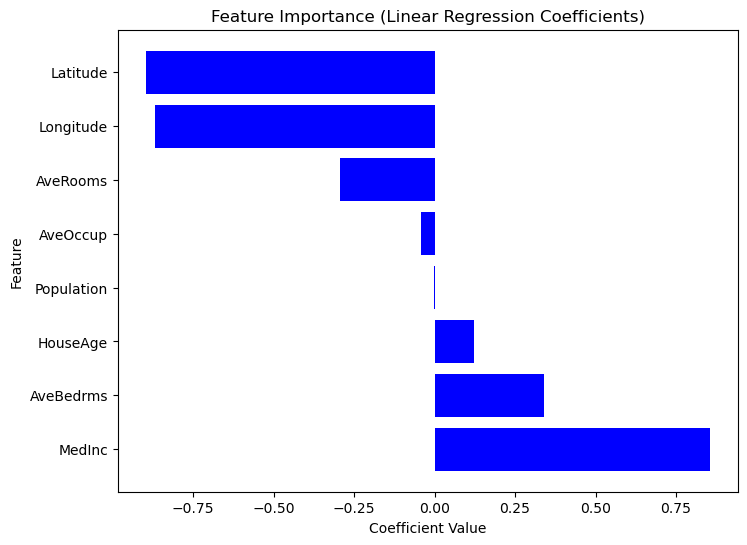

基于系数值的特征重要性图

接下来，我们来可视化残差与回归拟合。

# Compute residuals.
residuals = y_test - y_pred


# Create plots.
plt.figure(figsize=(12,5))


# Plot 1: Residuals Distribution.
plt.subplot(1,2,1)
sns.histplot(residuals, bins=30, kde=True, color="blue")
plt.axvline(x=0, color='red', linestyle='--')
plt.title("Residuals Distribution")
plt.xlabel("Residuals (y_actual - y_predicted)")
plt.ylabel("Frequency")


# Plot 2: Regression Fit (Actual vs Predicted).
plt.subplot(1,2,2)
sns.scatterplot(x=y_test, y=y_pred, alpha=0.5)
plt.plot([min(y_test), max(y_test)], [min(y_test), max(y_test)], color='red', linestyle='--')  # Perfect fit line
plt.title("Regression Fit: Actual vs Predicted")
plt.xlabel("Actual Prices (in $100,000s)")
plt.ylabel("Predicted Prices (in $100,000s)")


# Show plots.
plt.tight_layout()
plt.show()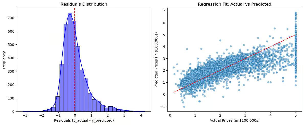

用于可视化残差与回归拟合的图表

残差分布图（左）应以 0 为中心，表明误差是随机分布的。若残差近似正态分布，模型拟合较好；若存在偏斜或趋势，可能意味着系统性误差。回归拟合图（右）对比真实值与预测值，红色虚线代表完美拟合。如果散点紧贴该线，预测较为准确；若出现某种模式（如曲线），则关系可能并非真正线性。 

这些可视化有助于诊断过拟合或欠拟合，揭示残差中的模式（提示遗漏的关系），并清晰评估模型的有效性。

真实世界的应用

线性回归在各行业被广泛用于预测与决策。在房地产中，它根据面积、位置等因素估算房价。 

在销售与市场领域，它用于需求预测与预算优化；医疗领域将其用于疾病风险评估；金融中用于股价预测与信用评分；制造领域用于质量控制与故障预测。 

何时使用线性回归

• 特征与目标变量之间呈线性关系。
• 可解释性与简洁性比复杂建模更重要。
• 数据只需最少的特征工程。

何时不宜使用线性回归

• 目标与特征之间关系复杂且非线性。
• 数据高度相关。
• 数据包含无法删除的离群点。在此情况下，您可能需要进行数据变换或采用策略减轻其影响。

总结

线性回归仍是机器学习与统计建模中最基础且最常用的技术之一。尽管简单，它是理解变量关系并在众多真实场景中进行预测的有力工具。

本教程的要点如下：

• 应用广泛。线性回归在多个行业与问题领域都能提供有价值的洞见。
• 易于解释。不同于复杂的“黑箱”模型，线性回归基于系数的解释清晰，便于理解与说明。
• 特征选择。合理的特征选择与多重共线性的处理，能确保模型保持准确、稳定与可靠。 

如需进一步了解 Python 字符串插值，请查看 DataCamp 的资源。

• 简单线性回归：您需要了解的一切 - 教程
• 如何在 R 中进行线性回归 - 教程
• Excel 中的线性回归：初学者的全面指南 - 教程
• R 中的回归入门 - 课程
• 使用 scikit-learn 的监督学习 - 课程
• Scikit-Learn 速查表：Python 机器学习 - 速查表
• 理解 Python 中的逻辑回归 - 教程