Sklearn Linear Regression: A Complete Guide with Examples

Linear regression is a fundamental technique in statistics and machine learning that helps model the relationship between variables. In simple terms, it allows us to predict an outcome based on one or more influencing factors. It is widely applied in real estate pricing, sales forecasting, risk assessment, and many other fields.

In this tutorial, we'll explore linear regression in scikit-learn, covering how it works, why it's useful, and how to implement it using scikit-learn. By the end, you'll be able to build and evaluate a linear regression model to make data-driven predictions.

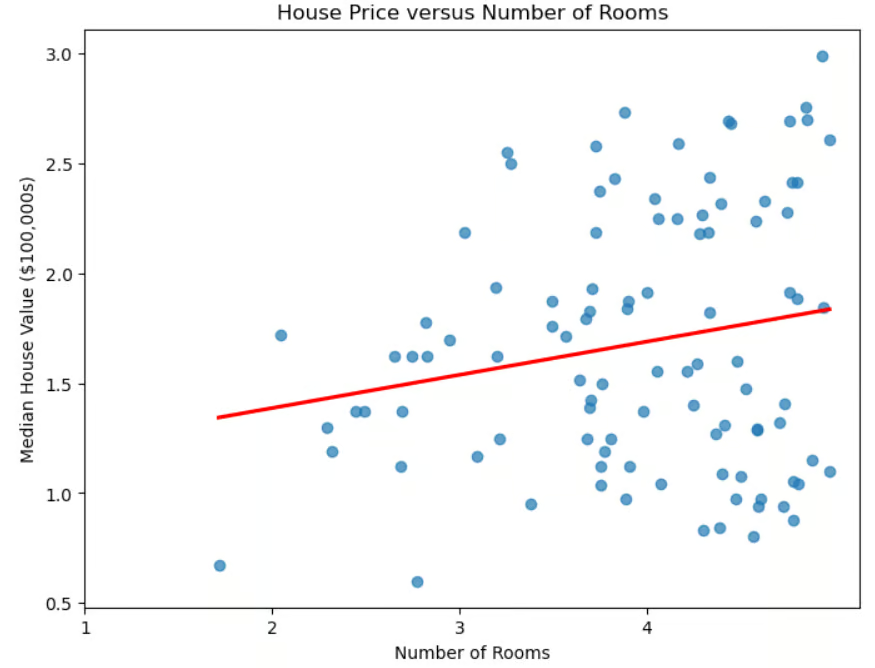
Scatter plot of House Price versus Number of Rooms

Linear regression and machine learning

Beyond its immediate usefulness in determining house prices, linear regression plays an important role in machine learning.

• It is a foundational model for understanding more advanced techniques like logistic regression, neural networks, and support vector machines.
• It is fast to train, making it ideal for rapid prototyping.
• It also serves as a baseline for comparison. If more advanced models don’t significantly outperform it, their added complexity may not be justified.
• Unlike some techniques (such as deep learning), it is easily interpretable.
• It can aid in feature selection, identifying the most useful predictors.

Despite its simplicity, linear regression remains an indispensable tool in machine learning due to its efficiency, interpretability, and versatility.

Linear regression and the scikit-learn library

The scikit-learn library makes linear regression easy to implement. This library has many advantages.

• It has a consistent interface. The code needed to implement different ML algorithms is similar.
• The code is simple, with complex math and implementation details extracted away. For instance to fit a model on training data, just use the line model.fit(X_train, y_train).
• It provides easy access to model coefficients.
• It provides built-in metrics to evaluate model performance.
• It is easy to integrate linear regression (or any other ML algorithm) with preprocessing steps, such as scaling and feature selections, using Pipeline.

If you’re new to scikit-learn, you can check out our course on Machine Learning with scikit-learn to get a hands-on introduction to the Python library. 

Understanding Linear Regression

As we have seen, in simple linear regression, the data is modeled using a "best-fit line." The formula for this line is: 

where m is the slope of the line and b is the intercept.

"Multiple linear regression" generalizes the case of one predictor to several predictors (number of rooms, proximity to the ocean, median income of the neighborhood). The formula is generalized to: 

where each x_i is an independent variable and the corresponding b_i is its coefficient. In three dimensions, the line is generalized to a plane. In higher dimensions, the plane becomes a "hyperplane."

How do we interpret the coefficients and the intercept? The intercept is the predicted value of y when all independent variables are 0, or put another way, is the baseline value of the dependent variable when there is no contribution from the predictors. Each coefficient b_i represents the change in the dependent variable y for a one-unit change in x_i, holding all other independent variables constant.

Setting Up the Environment

Installing scikit-learn is easy. Simply use the command pip install scikit-learn. If you wish to install a specific version, say 1.2.2, then modify the command to include the version: pip install scikit-learn==1.2.2. If you use Anaconda, scikit-learn should already be installed. If for some reason you still need to install it when using the Anaconda distribution, use the command conda install scikit-learn.

Several libraries are either necessary or recommended when using scikit-learn. The numpy library is needed for storing features and labels. The pandas library is recommended for loading, preprocessing and exploring datasets. 

If you're using scikit-learn, you're most likely using pandas already for your data prep. To plot your results, you'll likely use matplotlib or seaborn or both. Any of these libraries can be installed using pip install, similar to the example above. You can even install multiple libraries using one command:

pip install scikit-learn numpy pandas matplotlib seaborn.

Implementing Linear Regression in sklearn

Before we load the dataset, let's import the usual suspects.

# Import libraries.
import numpy as np
import pandas as pd
import matplotlib.pyplot as plt
import seaborn as sns

Loading the dataset

Let's use the well-known California housing dataset.

# Read in California housing dataset.
from sklearn.datasets import fetch_california_housing


housing = fetch_california_housing()

Preparing the data

Let's split the data into training and testing sets. We import the train_test_split() method from sklearn.model_selection, then invoke it, specifying a test set percentage, and a random_state. We'll also use simple linear regression, using the feature corresponding to the average number of rooms.

# Import train_test_split.
from sklearn.model_selection import train_test_split


# Create features X and target y.
X = pd.DataFrame(housing.data, columns=housing.feature_names)[["AveRooms"]]
y = housing.target  # Median house value in $100,000s


# Split the dataset into training (80%) and testing (20%) sets.
X_train, X_test, y_train, y_test = train_test_split(X, y, test_size=0.2, random_state=42)

Now that we've split the data into test and train sets, let's standardize features. This process ensures that all variables are on the same scale, which can improve model performance and numerical stability.

# Import StandardScaler.
from sklearn.preprocessing import StandardScaler

# Instantiate StandardScaler.
scaler = StandardScaler()

# Fit and transform training data.
X_train_scaled = scaler.fit_transform(X_train)

# Also transform test data.
X_test_scaled = scaler.transform(X_test)

In this code, StandardScaler is a data preprocessing tool used to remove the mean and scale features to unit variance. This helps prevent certain features from dominating the model due to differences in scale.

The scaler is fitted on the training data using the fit_transform() method. The test data is then transformed separately using the transform() method to ensure it is scaled using the same factors as the training data, preventing data leakage.

Training the linear regression model

To create a linear regression model, import LinearRegression() from sklearn.linear_model. Invoke it and assign it to a variable.

# Import LinearRegression.
from sklearn.linear_model import LinearRegression


# Instantiate linear regression model.
model = LinearRegression()

Fitting the model with training data is straightforward.

# Fit the model to the training data.
model.fit(X_train_scaled, y_train)

Making predictions

Now that we've trained our model, we make predictions on the test set.

# Make predictions on the testing data.
y_pred = model.predict(X_test_scaled)

Evaluating model performance

Now that we've made predictions on the test set, we need to know how well they match with reality. There are several metrics available to evaluate the performance of a regression algorithm. Some of the most common ones are the coefficient of determination (R²), mean squared error (MSE), and root mean squared error (RMSE).

The coefficient of determination, denoted R², measures how well a regression model explains the variability of the target variable. In other words, it quantifies how much of the variability in the target variable is explained by the predictors, known as the goodness of fit.

To further understand this, let's look at the formula:

where yactual is the actual values of the target variable, ypredicted is the predicted values from the model, and ȳ is the mean of the actual values. This formula helps us understand how much variance in the target variable is explained by the model. The denominator represents the total variance in the data, while the numerator represents the unexplained variance after applying the regression model. The ratio, therefore, gives the percentage of variance explained by the model.

How do we interpret R²?

• R² = 1: the model perfectly explains all the variance in the target variable. 
• R² = 0: the model explains none of the variance; predictions are no better than simply using the mean. 
• R² < 0: The model performs worse than simply using the mean, indicating a poor fit.

Some key considerations to keep in mind.

• Higher R² is not always better. A high R² may indicate overfitting, especially with complex models. 
• Adding more features can artificially increase R², so a higher value isn't necessarily better.
• For multiple regression, use adjusted R², which accounts for the number of predictors and avoids misleading improvements from unnecessary variables.

Evaluating model performance using the coefficient of determination is easy with scikit-learn.

# Import metrics.
from sklearn.metrics import mean_squared_error, r2_score


# Calculate and print R^2 score.
r2 = r2_score(y_test, y_pred)
print(f"R-squared: {r2:.4f}")

R-squared: 0.0138

Other commonly used metrics are the mean squared error (MSE) and the root mean squared error (RMSE). These metrics measure how far a model’s predictions deviate from the actual values.

MSE calculates the average squared difference between actual and predicted values: 

for the total number of observations n. Since the errors are squared before averaging, larger errors are more heavily penalized than smaller ones, making MSE sensitive to outliers. A lower MSE indicates a better model fit.

To address this issues, RMSE is used, which is simply the square root of MSE. Since RMSE is in the same units as the target variable, it provides a more interpretable measure of how far predictions are off, on average.

Calculating MSE and RMSE is easy with scikit-learn.

# Calculate and print MSE.
mse = mean_squared_error(y_test, y_pred)
print(f"Mean squared error: {mse:.4f}")


# Calculate and print RMSE.
rmse = mse ** 0.5
print(f"Root mean squared error: {rmse:.4f}")

Mean squared error: 1.2923
Root mean squared error: 1.1368

Working with Multiple Linear Regression in scikit-learn

Let's rerun the model using all of our available features, not just the average number of rooms. Do you expect better or worse results?

# Uses all features.
import numpy as np
import pandas as pd
import matplotlib.pyplot as plt
import seaborn as sns
from sklearn.datasets import fetch_california_housing
from sklearn.model_selection import train_test_split
from sklearn.preprocessing import StandardScaler
from sklearn.linear_model import LinearRegression
from sklearn.metrics import mean_squared_error, r2_score


# Load data set.
housing = fetch_california_housing()


# Split into X, y.
X = pd.DataFrame(housing.data, columns=housing.feature_names)
y = housing.target  # Median house value in $100,000s
X_train, X_test, y_train, y_test = train_test_split(X, y, test_size=0.2, random_state=42)


# Scale the data.
scaler = StandardScaler()


X_train_scaled = scaler.fit_transform(X_train)
X_test_scaled = scaler.transform(X_test)


# Create model and fit it to the training data.
model = LinearRegression()
model.fit(X_train_scaled, y_train)


# Make predictions.
y_pred = model.predict(X_test_scaled)


# Calculate and print errors.
r2 = r2_score(y_test, y_pred)
print(f"R-squared: {r2:.4f}")


mse = mean_squared_error(y_test, y_pred)
print(f"Mean squared error: {mse:.4f}")


rmse = mse ** 0.5
print(f"Root mean squared error: {rmse:.4f}")

R-squared: 0.5758
Mean squared error: 0.5559
Root mean squared error: 0.7456

We see the results are quite a bit better than when using only one feature. However, this raises the question of whether we need all the features. Are some features more relevant than others? Choosing the most relevant features from the dataset is known as feature selection.

Feature selection is important for a number of reasons.

• Reduces overfitting. Fewer features mean less complexity, reducing the risk of overfitting.
• Improves accuracy. Removing irrelevant or redundant features helps the model focus on meaningful patterns.
• Enhances interpretability. Makes models easier to understand by highlighting the most important factors.
• Speeds up training. Reducing the number of features decreases computational time and memory usage.

When multiple features are highly correlated, they are redundant, meaning that they are essentially giving the model the same information. This situation is referred to as multicollinearity. While multicollinearity doesn’t always impact the accuracy of predictive models, it complicates feature selection and interpretation, especially in linear regression and related models.

Variance Inflation Factor (VIF) is a metric used to detect multicollinearity among predictors. For each predictor, the VIF is calculated as: 

where R_i² is the R² value obtained when the predictor X_i is regressed against all other predictors in the model. A higher VIF means the predictor is highly correlated with other variables.

• VIF = 1: no multicollinearity (ideal scenario).
• VIF < 5: low to moderate multicollinearity (generally acceptable).
• VIF > 5: high multicollinearity (consider removing or combining correlated variables).
• VIF > 10: severe multicollinearity (strongly suggests variable redundancy).

# Import libraries.
import numpy as np
import pandas as pd
import seaborn as sns
import matplotlib.pyplot as plt
from sklearn.datasets import fetch_california_housing
from statsmodels.stats.outliers_influence import variance_inflation_factor


# Load the dataset.
housing = fetch_california_housing()
X = pd.DataFrame(housing.data, columns=housing.feature_names)


# Compute the correlation matrix.
corr_matrix = X.corr()


# Identify pairs of features with high collinearity (correlation > 0.8 or < -0.8).
high_corr_features = [(col1, col2, corr_matrix.loc[col1, col2])
                     for col1 in corr_matrix.columns
                     for col2 in corr_matrix.columns
                     if col1 != col2 and abs(corr_matrix.loc[col1, col2]) > 0.8]


# Convert to a DataFrame for better visualization.
collinearity_df = pd.DataFrame(high_corr_features, columns=["Feature 1", "Feature 2", "Correlation"])
print("\nHighly Correlated Features:\n", collinearity_df)


# Compute Variance Inflation Factor (VIF) for each feature.
vif_data = pd.DataFrame()
vif_data["Feature"] = X.columns
vif_data["VIF"] = [variance_inflation_factor(X.values, i) for i in range(X.shape[1])]


# Print VIF values.
print("\nVariance Inflation Factor (VIF) for each feature:\n", vif_data)

   Highly Correlated Features:
       Feature 1  Feature 2  Correlation
   0   AveRooms  AveBedrms     0.847621
   1  AveBedrms   AveRooms     0.847621
   2   Latitude  Longitude    -0.924664
   3  Longitude   Latitude    -0.924664
  
   Variance Inflation Factor (VIF) for each feature:
          Feature         VIF
   0      MedInc   11.511140
   1    HouseAge    7.195917
   2    AveRooms   45.993601
   3   AveBedrms   43.590314
   4  Population    2.935745
   5    AveOccup    1.095243
   6    Latitude  559.874071
   7   Longitude  633.711654

Let's remove AveBedrms from the model.

# Import libraries.
import numpy as np
import pandas as pd
import matplotlib.pyplot as plt
import seaborn as sns
from sklearn.datasets import fetch_california_housing
from sklearn.model_selection import train_test_split
from sklearn.preprocessing import StandardScaler
from sklearn.linear_model import LinearRegression
from sklearn.metrics import mean_squared_error, r2_score


# Load California housing dataset.
housing = fetch_california_housing()


# Create DataFrame and remove "AveBedrms" feature.
X = pd.DataFrame(housing.data, columns=housing.feature_names).drop(columns=["AveBedrms"])
y = housing.target  # Median house value in $100,000s


# Split data into training and testing sets.
X_train, X_test, y_train, y_test = train_test_split(X, y, test_size=0.2, random_state=42)


# Scale the data (Standardization).
scaler = StandardScaler()
X_train_scaled = scaler.fit_transform(X_train)
X_test_scaled = scaler.transform(X_test)


# Create a linear regression model and train it.
model = LinearRegression()
model.fit(X_train_scaled, y_train)


# Make predictions on the test set.
y_pred = model.predict(X_test_scaled)


# Calculate performance metrics.
r2 = r2_score(y_test, y_pred)
mse = mean_squared_error(y_test, y_pred)
rmse = np.sqrt(mse)
# Print evaluation metrics
print(f"R-squared: {r2:.4f}")
print(f"Mean squared error: {mse:.4f}")
print(f"Root mean squared error: {rmse:.4f}")

R-squared: 0.5823
Mean squared error: 0.5473
Root mean squared error: 0.7398

The results are (marginally) improved.

Extracting Model Insights

Building a regression model is just the first step; understanding its outputs is equally important. By analyzing the model's coefficients, we can determine which features have the most significant impact on predictions.

Understanding regression coefficients

Once a linear regression model is trained, the coefficients can be accessed using model.coef_. The intercept can be accessed using model.intercept_.

Once a linear regression model is trained using LinearRegression(), the coefficients can be accessed using model.coef_ and the intercept can be accessed using model.intercept_.

print("Intercept:", model.intercept_)


coeff_df = pd.DataFrame({"Feature": X.columns, "Coefficient": model.coef_})
print("\nFeature Coefficients:\n", coeff_df)

   Intercept: 2.0719469373788777  

   Feature Coefficients:

         Feature  Coefficient

   0     MedInc     0.725747

   1   HouseAge     0.121519

   2   Latitude    -0.943105

   3  Longitude    -0.900735

Summarizing model results

Since Scikit-Learn does not provide a built-in summary() method like Statsmodels, we can manually extract and visualize the importance of each feature using regression coefficients. Features with larger absolute coefficients have a stronger impact on the target variable. Consider the following code.

# Sort dataframe by coefficients.
coef_df_sorted = coef_df.sort_values(by="Coefficient", ascending=False)


# Create plot.
plt.figure(figsize=(8,6))
plt.barh(coef_df["Feature"], coef_df_sorted["Coefficient"], color="blue")
plt.xlabel("Coefficient Value")
plt.ylabel("Feature")
plt.title("Feature Importance (Linear Regression Coefficients)")
plt.show()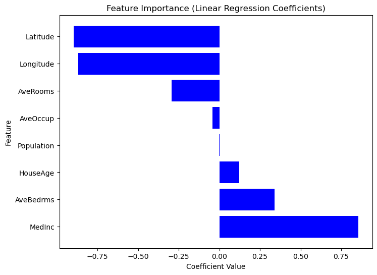

Graph of Feature Importance Based on Coefficient Values

Now, let's visualize residuals and the regression fit.

# Compute residuals.
residuals = y_test - y_pred


# Create plots.
plt.figure(figsize=(12,5))


# Plot 1: Residuals Distribution.
plt.subplot(1,2,1)
sns.histplot(residuals, bins=30, kde=True, color="blue")
plt.axvline(x=0, color='red', linestyle='--')
plt.title("Residuals Distribution")
plt.xlabel("Residuals (y_actual - y_predicted)")
plt.ylabel("Frequency")


# Plot 2: Regression Fit (Actual vs Predicted).
plt.subplot(1,2,2)
sns.scatterplot(x=y_test, y=y_pred, alpha=0.5)
plt.plot([min(y_test), max(y_test)], [min(y_test), max(y_test)], color='red', linestyle='--')  # Perfect fit line
plt.title("Regression Fit: Actual vs Predicted")
plt.xlabel("Actual Prices (in $100,000s)")
plt.ylabel("Predicted Prices (in $100,000s)")


# Show plots.
plt.tight_layout()
plt.show()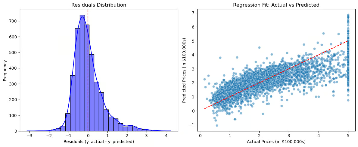

Plots to Visualize Residuals and Regression Fit

The residuals distribution (left plot) should be centered around zero, indicating that errors are randomly distributed. If the residuals follow a normal distribution, the model fits well, but if there is skewness or a trend, it may suggest systematic errors. The regression fit (right plot) compares actual vs. predicted values, with the red dashed line representing a perfect fit. If points closely follow the line, predictions are accurate, but if a pattern (e.g., a curve) appears, the relationship may not be truly linear. 

These visualizations help diagnose overfitting or underfitting, reveal patterns in residuals that suggest missing relationships, and provide a clear assessment of the model's effectiveness.

Real-World Applications

Linear regression is widely used across industries for prediction and decision-making. In real estate, it estimates house prices based on factors like size and location. 

Sales and marketing use it for demand forecasting and budget optimization, while healthcare applies it to disease risk assessment. In finance, it aids in stock price prediction and credit scoring, and in manufacturing, it helps with quality control and failure prediction. 

When to use linear regression

• Features and the target variable have a linear relationship.
• Interpretability and simplicity matter more than complex modeling.
• Data requires minimal feature engineering.

When not to use linear regression

• The relationship between the target and the features is complex and non-linear.
• Data is highly correlated.
• The data contains outliers that cannot be removed. In this case, you may need to apply data transformations or use strategies to mitigate their impact.

Conclusion

Linear regression remains one of the most fundamental and widely used techniques in machine learning and statistical modeling. Despite its simplicity, it is a powerful tool for understanding relationships between variables and making predictions in various real-world applications.

Here are the key takeaways from the tutorial:

• Versatile applications. Linear regression provides valuable insights across multiple industries and problem domains.
• Interpretable.  Unlike complex black-box models, linear regression offers clear coefficient-based interpretations, making it easy to interpret and explain.
• Feature selection. Properly selecting features and addressing multicollinearity ensures that models remain accurate, stable, and reliable. 

For further information on Python string interpolation, check out DataCamp's resources.

• Simple Linear Regression: Everything You Need to Know - Tutorial
• How to Do Linear Regression in R - Tutorial
• Linear Regression in Excel: A Comprehensive Guide For Beginners - Tutorial
• Introduction to Regression in R - Course
• Supervised Learning with scikit-learn - Course
• Scikit-Learn Cheat Sheet: Python Machine Learning - Cheat Sheet
• Understanding Logistic Regression in Python - Tutorial