
Our biggest-ever sale. 60% off AI & data skills
Buy Now
Now, let's explore some additional techniques for creating specific varieties of clustered column charts in Excel.
What if we want to change the clustering (grouping) criterion for our chart?
By default, each group of columns refers to a specific category from the column containing category names. In contrast, each column in a group of columns represents a particular type of item taken from the corresponding column header.
However, in some cases, we may want to swap the categories with the types of items.
Returning to our cats, dogs, and hamsters example, let's say that we need to cluster them by animal type rather than by pet shop:
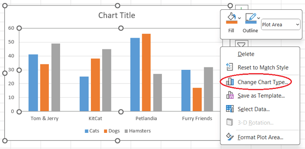
Opening the Change Chart Type window. Image by Author
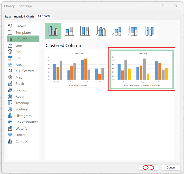
Changing the clustering criterion for a clustered column chart. Image by Author
Creating a 3D variant of a clustered column chart in Excel is as easy as making a regular one:
Remember, though, that creating 3D clustered column charts isn't considered a good practice, as discussed further in the section on “Best Practices for Clustered Column Charts.”
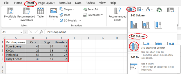
Creating a 3D clustered column chart. Image by Author
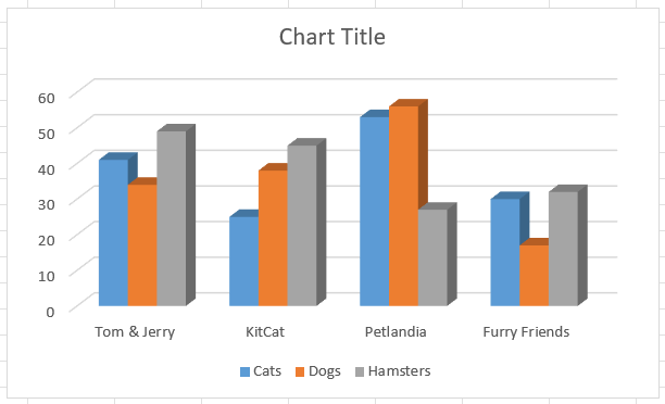
A 3D clustered column chart. Image by Author
Sometimes, we may want to combine a clustered column chart with a line chart on a single visual. This type of chart is called a combo chart or a combination chart.
A combo chart is commonly used to show the evolution of different types of data over the same period.
Therefore, our table with sold pets isn't the best use case for creating a combo chart since it doesn't contain either a time series or data types that are different by nature (such as sales and prices).
Let's use it anyway for learning purposes to see how we can build a clustered column and line combo chart in Excel:
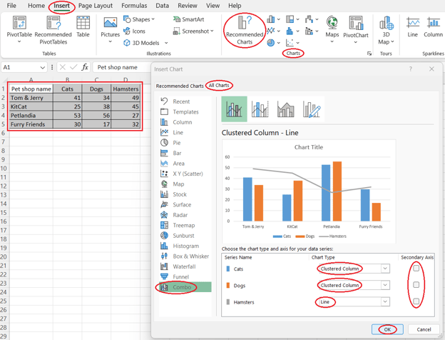
Creating a clustered column and line combo chart. Image by Author
Consider taking the Excel Fundamentals skill track to fully utilize Excel for visualizing and analyzing data.
Let's outline some best practices for creating clustered column charts in Excel.
Fortunately, Excel takes care of many of them by default, including adding an automatic legend, avoiding redundant elements, opting for a colorblind-friendly palette, starting the y-axis from zero, and making clustering obvious.
For the others, or if you want to adjust the defaults manually, it's recommended to follow the below practices to avoid typical caveats:
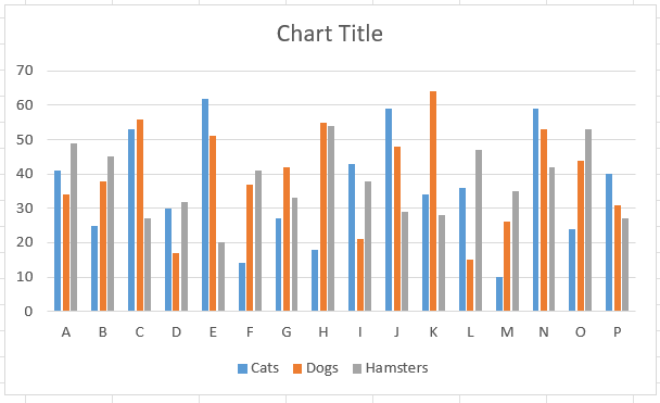
A clustered column chart with too many clusters. Image by Author
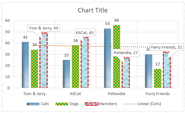
A clustered column chart with redundant elements. Image by Author
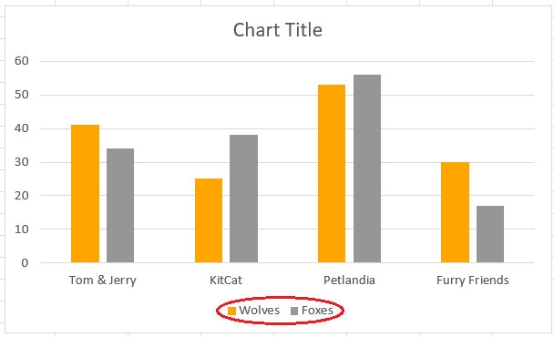
A clustered column chart with counterintuitive colors. Image by Author
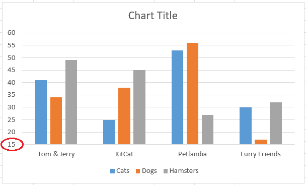
A clustered column chart with a cut y-axis. Image by Author
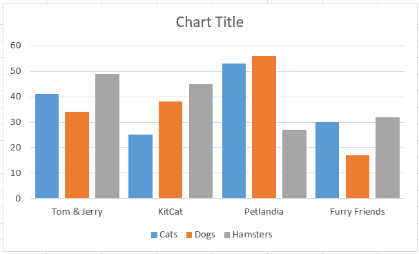
A clustered column chart with unobvious clustering. Image by Author
To wrap up, this article discussed what a clustered column chart is, its purpose, its key features, and why Excel is a good choice for creating this type of plot.
We also explored how to create and customize a clustered column chart in Excel, including its specific types and what best practices to follow when making them.
If you enjoyed this article, you may find the Data Visualization in Excel and Data Analysis in Excel courses helpful for continued learning.
Yes, you can create a clustered column chart with non-adjacent data columns. To do this, hold down the Ctrl key while selecting the different columns you want to include in your chart.
To add data labels, click on one of the columns in the chart, then right-click and select "Add Data Labels." This will add the values directly onto each column, making it easier to see the exact figures.
Yes, you can add a secondary axis. This is useful if you have data series with different scales. To add a secondary axis, select the data series you want to change, right-click, choose "Format Data Series," and then select "Secondary Axis" in the format pane.
Starting the y-axis from zero is important because it accurately represents the relative size of the data values. Cutting the y-axis can distort the visual interpretation of the data, making differences appear more significant than they are.
To avoid clutter, try to limit the number of data series and clusters. If you have too many, consider breaking your data into multiple charts or using filters to display specific data series at a time.

Учебное руководство
 Oluseye Jeremiah• 8 мин

Учебное руководство
 Joleen Bothma• 12 мин

Учебное руководство
 Aditya Sharma• 12 мин
Learn more about Excel with these courses!
Курс
Научитесь анализировать данные с помощью PivotTables и промежуточных логических функций, а затем перейдите к инструментам вроде what-if analysis и forecasting.
Курс
Научитесь создавать разные визуализации в Excel для разных макетов данных, применяя лучшие практики для создания дашбордов.
Курс
Освойте подготовку данных Excel с помощью логических функций, вложенных формул, функций поиска и сводных таблиц.


Clustered column charts are among the most helpful and, hence, commonly used types of charts. Because of their popularity, they can be created in virtually all programs and software geared toward data analysis, and Excel is no exception.
In this article, we'll learn what a clustered column chart is and how to create and customize it in Excel. Besides, we'll cover some additional techniques and best practices for clustered column charts in Excel.
For a quick start or refresher on Excel, check out the Learn Excel course.
The Quick Answer: How to Create a Clustered Column Chart in Excel
To create a clustered column chart in Excel, follow these steps:
What Is a Clustered Column Chart and What Is It Used for?
A clustered column chart, also known as a grouped bar chart, is a visualization that displays the discrete values for two or more types of items by category.
Such values are shown as vertical rectangular columns, the height of each column corresponding to the value it represents. These vertical columns are clustered by category, and all data series (types of items) share the same x-axis labels since the categories are the same for each.
Each cluster of columns represents a specific category, while each column in a cluster represents a certain type of items.
Clustered column charts compare different data series, each corresponding to a distinct type of item, category-wise.
Features of Clustered Column Charts
A clustered column chart is characterized by two main features:
To learn or revise different types of data visualizations in Excel and to fully leverage the tool's power, feel free to explore the Visualizing Data in Excel tutorial.
Why Excel Is Good For Creating Clustered Column Charts
There are numerous advantages of using Excel for creating clustered column charts:
How to Create and Customize a Clustered Column Chart in Excel
Now that we know what a clustered column chart is and why Excel is suitable for creating it, let's see how we can build and format a basic clustered column chart in Excel.
Throughout this and the next section, we're going to work with the table below, which contains the names of fictitious pet shops and the number of cats, dogs, and hamsters each of them sold during a certain period.
An example Excel table with pets sold by fictitious pet shops. Image by Author
It goes without saying that before building a clustered column chart in Excel, it's important to properly clean and transform your data using suitable methods and best practices. Check out the Data Preparation in Excel course to learn more about this.
Creating a clustered column chart
To create a clustered column chart in Excel, you need to take four simple steps:
Selecting the data and opening the Insert Column or Bar Chart feature. Image by Author
Opening the Clustered Column option. Image by Author
Customizing a clustered column chart
Excel offers numerous ways of adjusting visuals. Many apply to all types of Excel charts, such as adding or removing chart elements or filters, changing the chart style or color scheme, customizing text, and moving the legend.
You can learn more in the tutorial on How to Create and Format a Combo Chart in Excel, in the chapter “How to Format a Combo Chart” in Excel.
In this section, we'll focus on the ways of formatting the data series constituting our clustered column chart.
Note: if you want to format only one column of a data series, e.g., for highlighting a column among the others, click twice, with a little delay on that column and then follow the above instructions.
Opening the Format Data Series pane. Image by Author
Adjusting the fill settings. Image by Author
Adjusting the border settings. Image by Author