IFS() Excel: Learn to Simplify Multiple Conditions

If you’ve ever tried to build a complex logic formula in Excel, you know how messy it can get with. The most difficult thing with nested IF() statements is trying to figure out which condition goes where.

That's why Excel introduced a new function called IFS(). It’s a cleaner and simpler way to check multiple conditions without tying yourself in knots. I’ll walk you through how IFS() works, with examples and tips to help you use it confidently.

What Is the IFS() Function in Excel?

The IFS() function helps us check multiple conditions simultaneously. It looks through each condition in the order you write them, and gives you the result for the first one that's TRUE.

So it’s an easier way to write what used to be a messy set of nested IF() formulas. Instead of stacking multiple IF() functions inside each other, IFS() lists all your conditions in one place. In total, you can add up to 127 condition-result pairs, although I doubt you will ever need so many conditions.

How the IFS() function works

Its syntax is:

=IFS(logical_test1, value_if_true1, [logical_test2, value_if_true2]…)

Here:

• logical_test1 (required) is the first condition.

• value_if_true1(required) return the results if logical_test1 is TRUE.

• The remaining 126 logical_test and value_if_true arguments are optional.

How to Use Excel IFS()

The IFS() function returns different results based on conditions. You can use logical operators like =, <, >, <=, and >= to build your logic. Here’s how to get started.

Option 1: Use the Formula Wizard

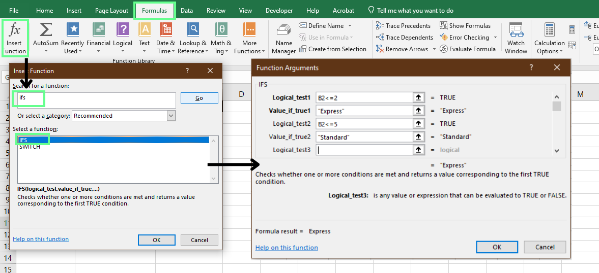
To use a Formula Wizard: 

1. Click the cell where you want your formula.

2. Go to the Formulas tab and choose Insert Function.

3. In the search box, type IFS and click Go.

4. Select IFS, click OK, then enter your conditions and results.

5. Click OK again to apply the formula.

This is a quick way to build a formula without typing it out yourself.

Use the Formula Wizard to apply the IFS() function. Image by Author.

Option 2: Write it manually

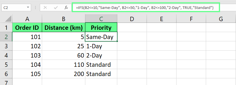
You can also write the formula manually. This is probably what most people do. All you have to do is type =IFS( in the cell and build your logic step by step. Suppose you’re assigning shipping methods based on delivery time:

• If it’s 2 days or less, that would be Express

• If it’s 3 to 5 days, that would be Standard

For this, here's the formula:

=IFS(B2<=2, "Express", B2<=5, "Standard")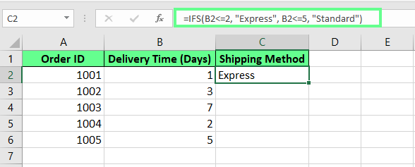

Apply the IFS() formula in a cell. Image by Author.

You can also copy your formula to other cells. To do so, drag the small square in the bottom corner of the cell (the fill handle). This will apply the formula down the column. Or just double-click it to fill automatically based on your data.

Pro Tip: Excel automatically updates the cell references when you copy a formula. If you want to keep a reference fixed, turn it into an absolute reference by pressing F4 (it changes A1 to $A$1).

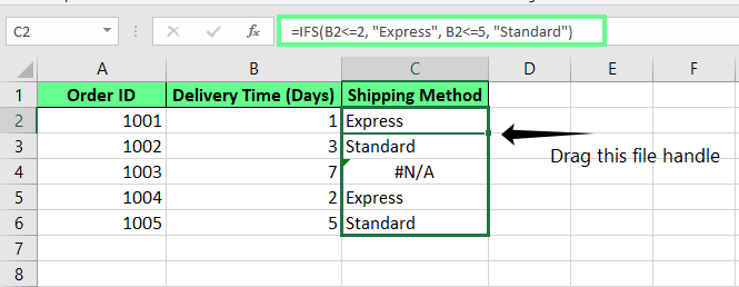
Copy down the formula using a file handle. Image by Author

But it throws an #N/A error in one cell because none of the conditions are met. To fix that, add a final condition using TRUE at the end of the formula. This works like a backup plan; it catches anything that didn’t match earlier and gives you a default result instead. 

=IFS(B2<=2, "Express", B2<=5, "Standard", TRUE, "Economy")

This removes the #N/A error and returns the default value.

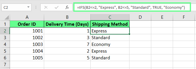
Handle #N/A error using the final ELSE condition. Image by Author.

Examples of the IFS() in Action

Now let's see some real-world examples, where most people use this function.

Grade assignment

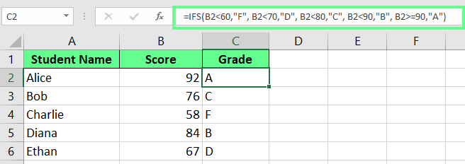
You can use IFS() to convert students’ scores into letter grades. Suppose you have a list of students and their test scores. You can use this formula to turn those numbers into grades:

=IFS(C5<60,"F", C5<70,"D", C5<80,"C", C5<90,"B", C5>=90,"A")

Here’s what it does:

• If the score is less than 60, it gives an F.

• If it’s less than 70, it gives a D.

• If it’s less than 80, that’s a C.

• If it’s less than 90, you get a B.

• If it’s 90 or more, that’s an A.

Excel checks each condition in order, and stops as soon as it finds one that’s TRUE. Even if more than one condition could apply, only the first match counts.

Assign grades to students using IFS(). Image by Author.

Error handling with TRUE

You can also use IFS() to show a custom message based on different status codes instead of letting Excel show a #N/A error. For example, if you have a list of codes and you want to show a message based on each one, here’s a formula you could use:

=IFS(A2=100,"OK", A2=200,"Warning", A2=300,"Error", TRUE,"Invalid")

Here’s how it works:

• If the code is 100, it shows OK.

• If it’s 200, it shows Warning.

• If it’s 300, it shows Error.

• If it doesn’t match any of those, it shows Invalid.

That last part is important. It will display the message based on the code. If no exact matches are found, the last condition TRUE acts as a fallback and returns Invalid.

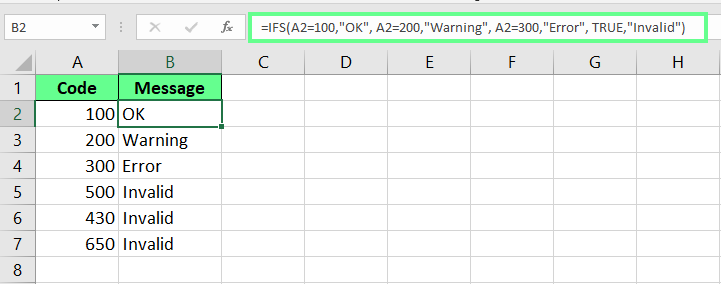
Show a message based on the code using the IFS() function. Image by Author.

Conditional text labels

You can also use IFS() to sort items into categories like fruits, vegetables, or drinks to keep track as new ones are added.

Here’s a simple formula to do this:

=IFS(A2="Grapes","Fruit", A2="Broccoli","Green Vegetable", A2="Tea","Beverage", TRUE,"Misc")

This is what it does:

• If the item is Grapes, it shows Fruit.

• If it’s Broccoli, it shows Green Vegetable.

• If it’s Tea, it shows Beverage.

• If it doesn’t match any of those, it shows Misc.

That last line (with TRUE) is your backup option. It catches anything that doesn’t fit the other categories.

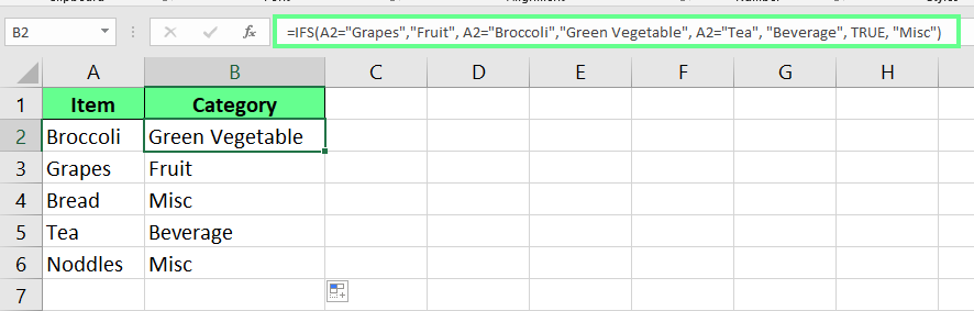
Categorize the item using IFS(). Image by Author.

Financial modeling

We can also use IFS() for financial modeling purposes. Let’s look at two common examples:

Apply discount tiers

You can use IFS() to assign a discount based on a customer's total purchase amount.

=IFS(B2>=500,"20% Discount", B2>=300,"10% Discount", B2>=100,"5% Discount", TRUE,"No Discount")

Here’s how it works:

• If the amount is equal to or greater than 500, it returns 20% Discount

• If the amount is equal to or greater than 300, it returns 10% Discount.

• If the amount is equal to or greater than 100, it returns 5% Discount.

• If the amount is less than 100, the final TRUE condition returns No Discount.

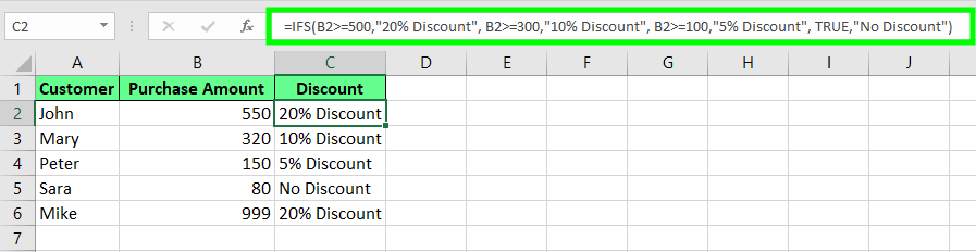
Apply discounts using IFS(). Image by Author.

Calculate leave days

You can also calculate how many leave days an employee is eligible for, based on how long they have been with the company. To do so, use the following formula:

=IFS(B2>=10,"30 Days", B2>=5,"20 Days", B2>=1,"10 Days", TRUE,"No Leave")

Here’s how it breaks down:

• 10 or more years means 30 Daysleave.

• 5 to 9 years means 20 Days.

• 1 to 4 years means 10 Days.

• Less than 1 year means No Leave.

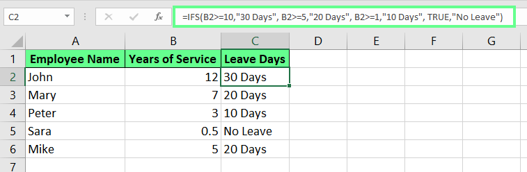
Assign leave days based on years of service using IFS(). Image by Author.

Data conversion

You can also use IFS() to convert file sizes from bytes into more readable units like KB, MB, or GB:

=IFS(B2<1024, B2 & " Bytes", B2<1048576, ROUND(B2/1024,1) & " KB", B2<1073741824, ROUND(B2/1048576,1) & " MB", TRUE, ROUND(B2/1073741824,1) & " GB")

This formula shows:

• Bytes for values under 1024

• KB for values under 1 MB

• MB for values under 1 GB

• GB for anything larger

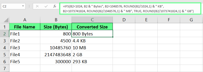
Convert file size from bytes to KB, MB, GB using IFS(). Image by Author.

IFS() vs. IF() vs. Nested IF()

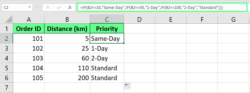
When working with multiple conditions in Excel, you have three options: IF(), nested IF(), or the IFS() function. Each one works differently, so here’s how to choose the right one.

Comparison in readability

If you're only checking one or two conditions, the basic IF() function is perfect. It's quick, simple, and gets the job done. But things get tricky when you try to check multiple conditions. That’s when we start stacking IF() functions inside each other, which makes the formula harder to read and even harder to change later.

Here’s an example:

=IF(A1<60,"F",IF(A1<70,"D",IF(A1<80,"C",IF(A1<90,"B","A"))))

It works, but it’s not easy to follow. All those brackets make it challenging to read and update.

Nested IF() is hard to read and understand. Image by Author. 

Now look at the same logic using IFS() instead:

=IFS(A1<60,"F", A1<70,"D", A1<80,"C", A1<90,"B", A1>=90,"A")

This one looks much simpler. Each condition is paired directly with a result without any nesting and bracket overload. So, if you want a formula that's easy to read, understand, and fix later, IFS() is a great choice.

IFS() is much easier to read and understand. Image by Author.

Performance considerations

The IFS() function checks every condition you give it, even if it has already found a match. So if you list five conditions, Excel still evaluates all five.

But nested IF() functions are a bit smarter. They use “short-circuiting,” which means they stop checking as soon as they find the first TRUE condition. That saves a little time in large spreadsheets with lots of formulas.

Quick comparison: When to use what

Here’s a quick tabular comparison to help you understand when to use IF(), nested IF(), and IFS():

IFS vs. SWITCH()

IFS() and SWITCH() both check multiple conditions in a single self-contained formula, but they work in different ways. Here’s a detailed comparison between both:

Things to Consider

You should keep a few things in mind when working with the IFS() function in Excel.

Common errors and how to fix them

First, let's see some common errors you may run into.

Too few arguments

If we add a condition but forget to include what should happen if it’s true (value_if_true). Excel shows a pop-up: "You've entered too few arguments for this function."

#N/A error

#N/A error will occur when none of the conditions in the formula are TRUE. Excel needs at least one to match, or it gets stuck. If you don't want to display #N/A , add TRUE at the end with a fallback value.

#VALUE! Error

#VALUE! error shows up when a logical_test argument doesn’t return a clear TRUE or FALSE. Maybe it’s a typo, or maybe the condition isn’t quite right. Either way, Excel won’t know what to do with it, so double-check your logic.

Tips and best practices

Now, here are a few best practices to make your formulas better and simpler: 

• Try to keep things simple. Ten or fewer conditions are usually enough.

• Add a fallback condition using TRUE as your last condition. It covers any cases that don’t meet your main conditions.

• Make sure every condition has a result, and that your tests are giving back either TRUE or FALSE.

• Test your formula with edge cases like 0, 100, or even blank cells to make sure it handles everything the way you expect.

Pros and cons

IFS() has some real benefits, but there are a few things to watch out for, too.

Final Thoughts 

The IFS() function is a handy way to check lots of conditions without your formula getting messy. It’s easier to read than multiple IF() statements stacked within each other and makes your logic much clearer. Make sure you list your conditions in the right order, and always add a final fallback using TRUE — that way, your formula won’t break if nothing matches.

If your logic is predictable and follows clear rules, IFS() is a great way to keep your spreadsheet neat and easy to manage.