Course
Introduction to Deep Learning in Python
4 hr
263.5K
In the Training Script portion, you'll be working on image super-resolution problem using a novel deep learning architecture. The task at hand would be to do a non-linear mapping from a low-field 3-Tesla Brain MR Image to a high-field 7-Tesla Brain MR Image. In this Testing Script portion, you will be using the weights that were trained in Part-1 and will predict on the unseen trained data. You'll also learn how to finally save the 2D images as a combined volume.
The tutorial is divided into two parts, the first part will walk you through the training process and the second part will cover the testing process.
Note: You would probably be interested in reading the paper if so, you can find the article here.
In a nutshell, you'll address the following topics in Part-1 of the tutorial:
Before you start following along with this tutorial make sure you have the exact same module versions as stated below:
Note: Before you begin, please note that the model will be trained on a system with Nvidia 1080 Ti GPU Xeon e5 GeForce processor with 32GB RAM. If you are using Jupyter Notebook, you will need to add three more lines of code where you specify CUDA device order and CUDA visible devices using a module called os.
In the code below, you set environment variables in the notebook using os.environ. It's good to do the following before initializing Keras to limit Keras backend TensorFlow to use the first GPU. If the machine on which you train on has a GPU on 0, make sure to use 0 instead of 1. You can check that by running a simple command on your terminal: for example, nvidia-smi
import os
os.environ["CUDA_DEVICE_ORDER"]="PCI_BUS_ID"
os.environ["CUDA_VISIBLE_DEVICES"]="0" #model will be trained on GPU
First, you import all the required modules like tensorflow, numpy and most importantly keras and the required functions or layers like Input, Conv2D,MaxPooling2D etc. since you'll be using all these frameworks for training the model!
In order to read the nifti format images, you also have to import a module called nibabel.
import os
import numpy as np
import math
import tensorflow as tf
import nibabel as nib
import numpy as np
from keras.layers import Input,Dense,merge,Reshape,Conv2D,MaxPooling2D,UpSampling2D
from keras.layers.normalization import BatchNormalization
from keras.models import Model,Sequential
from keras.callbacks import ModelCheckpoint
from keras.optimizers import RMSprop
from keras import backend as K
import scipy.misc
from sklearn.utils import shuffle
from sklearn.cross_validation import train_test_split
import matplotlib.pyplot as plt
from keras.models import model_from_json
Using TensorFlow backend.
/usr/local/lib/python3.5/dist-packages/sklearn/cross_validation.py:41: DeprecationWarning: This module was deprecated in version 0.18 in favor of the model_selection module into which all the refactored classes and functions are moved. Also, note that the interface of the new CV iterators is different from that of this module. This module will be removed in 0.20.
  "This module will be removed in 0.20.", DeprecationWarning)
The brain MRI 3T and 7T dataset consists of 3D volumes each volume has in total 207 slices/images of brain MRI's taken at different slices of the brain. Each slice is of dimension 173 x 173. The images are single channel grayscale images. There are in total 39 subjects, each subject containing the MRI scan of a patient. The image format is not jpeg, png, etc. but rather a nifti format. You will see in a later section on how to read the nifti format images.
The dataset consists of T1 modality MR images, T1 sequences are traditionally considered good for evaluation of anatomic structures. The dataset on which you will be working today consists of 3T and 7T Brain MRI's.
The dataset is public and is available for download at this source.
28 subjects are used for training while the remaining 11 subjects will be used for testing purpose.
Let's first define the dimensions of the data. You'll resize the image dimension from 173x173 to 176x176 in the data reading part. Here you will also define the data directory, the batch size for training the model, the number of channels, an Input() layer, train, and test matrices as a list and finally for rescaling you will load the text file which has the minimum and maximum values of the MRI dataset.
Note: For rescaling, you can also take the maximum and minimum of the dataset since you will not have the maxANDmin.txt file.
x,y = 173,173
full_z = 207
resizeTo=176
batch_size = 32
inChannel = outChannel = 1
input_shape=(x,y,inChannel)
input_img = Input(shape = (resizeTo, resizeTo, inChannel))
inp = "ground3T"
out = "ground7T"
train_matrix = []
test_matrix = []
min_max = np.loadtxt('maxANDmin.txt')Next, you load the mri data using the nibabel library and resize the images from 173 x 173 to 176 x 176 by padding zeros in x and y dimension.
Note that when you load a Nifti format volume, Nibabel does not load the image array. It waits until you ask for the array data. The standard way to ask for the array data is to call the get_data() method.
Since you want the 2D slices instead of 3D, you will use the train and test lists that you initialized before; every time you read a volume, you will iterate over all the complete 207 slices of the 3D volume and append each slice one by one into a list.
folder = os.listdir(inp)
Let's first load the 3T data.
for f in folder:
    temp = np.zeros([resizeTo,full_z,resizeTo])
    a = nib.load(inp + f)
    a = a.get_data()
    temp[3:,:,3:] = a
    a = temp
    for j in range(full_z):
        train_matrix.append(a[:,j,:])
Then, load the 7T data, and you use the same folder variable for loading 7T data as well since the number of 3T and 7T MR volumes are equal.
for f in folder:
    temp = np.zeros([resizeTo,full_z,resizeTo])
    b = nib.load(out + f)
    b = b.get_data()
    temp[3:,:,3:] = b
    b = temp
    for j in range(full_z):
        test_matrix.append(b[:,j,:])
Since train and test matrices is a list, you will use numpy module to convert the list into a numpy array.
Further, you will convert the type of the numpy array as float32 and also rescale both the input and the ground truth.
train_matrix = np.asarray(train_matrix)
train_matrix = train_matrix.astype('float32')
m = min_max[0]
mi = min_max[1]
train_matrix = (train_matrix - mi) / (m - mi)

test_matrix = np.asarray(test_matrix)
test_matrix = test_matrix.astype('float32')
test_matrix = (test_matrix - mi) / (m - mi)
Let's quickly print the shape of train_matrix (3T) and test_matrix (7T) matrices. They should have 28 x 207 = 5796 images in total, each having a dimension of 176 x 176.
train_matrix.shape
(5796, 176, 176)
test_matrix.shape
(5796, 176, 176)
Next, you will create two new variables augmented_images(3T/input) and Haugmented_images (7T/ground truth) of the shape train and test matrix. This will be a 4D matrix in which the first dimension will be the total number of images, second and third being the dimension of each image and last dimension being the number of channels which is one in this case."
augmented_images=np.zeros(shape=[(train_matrix.shape[0]),(train_matrix.shape[1]),(train_matrix.shape[2]),(1)])
Haugmented_images=np.zeros(shape=[(train_matrix.shape[0]),(train_matrix.shape[1]),(train_matrix.shape[2]),(1)])
Then you will iterate over all the images one by one, each time you will reshape the train and test matrix to 176 x 176 and append it to augmented_images(3T/input) and Haugmented_images (7T/ground truth) respectively.
for i in range(train_matrix.shape[0]):
    augmented_images[i,:,:,0] = train_matrix[i,:,:].reshape(resizeTo,resizeTo)
    Haugmented_images[i,:,:,0] = test_matrix[i,:,:].reshape(resizeTo,resizeTo)
After all of this, it's important to partition the data. In order for your model to generalize well, you split the data into two parts: a training and a validation set. You will train your model on 80% of the data and validate it on 20% of the remaining training data.
This will also help you in reducing the chances of overfitting, as you will be validating your model on data it would not have seen in the training phase.
You can use the train_test_split module of scikit-learn that you had defined in the begining to divide the data properly:
data,Label = shuffle(augmented_images,Haugmented_images, random_state=2)
X_train, X_test, y_train, y_test = train_test_split(data, Label, test_size=0.2, random_state=2)
X_test = np.array(X_test)
y_test = np.array(y_test)
X_test = X_test.astype('float32')
y_test = y_test.astype('float32')
X_train = np.array(X_train)
y_train = np.array(y_train)
X_train = X_train.astype('float32')
y_train = y_train.astype('float32')
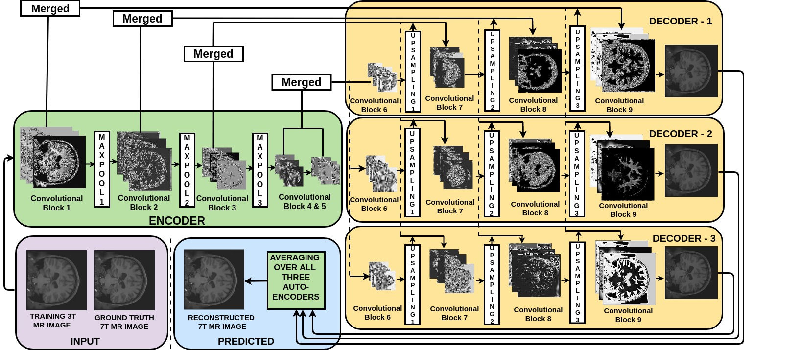
Next, you define the proposed architecture with blocks of subsequent filter layers followed by a max pooling layer in the encoder section as shown in next cell. To reconstruct the original size of an image at output, an upsampling layer is introduced in each block of the decoders. While upsampling, there may be some artifacts introduced due to missing details in the downsampled input of decoder. Hence, you concatenate the input of decoder with its upscaled version from the encoder in order to provide the nature of upscaled details for better reconstruction while upsampling in decoder. Indeed, adding the merge connections will yield a significant PSNR improvement (of the order of 5db). This setting of our architecture is inspired by this paper.
The proposed approach employs a single encoder and multiple decoder architecture with a single channel input. Three convolutional layers are used in each block of an encoder and all the three decoders, followed by a batch normalization layer to maintain the numerical stability.
The first convolutional block in the encoder has 32 filters, and the number of filters doubles after each convolutional block. In all the decoders the first convolutional block has 256 filters, and the number of filters are halved after each block. You will use a filter size of 3-by-3 in all convolutional blocks.
Rectified Linear Unit (ReLU) will be used as an activation function in all the layers except the final layer. Since data is normalized between 0 and 1, a Sigmoid activation function is used at the final layer.
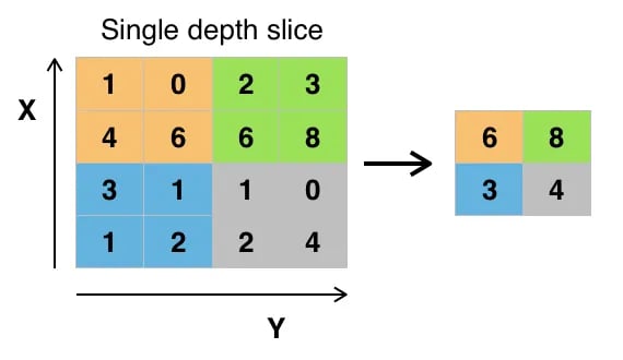
It is well known that local image details at various scales play a significant role in image reconstruction. The proposed architecture considers images at different scales using hierarchical layers for downsampling (maxpooling) and upsampling (each for a factor of 2) in encoder and decoders, respectively. The encoded representation obtained after three downsampling operations brings the data from a high dimension input to a latent space representation.
def encoder(input_img):
    conv1 = Conv2D(32, (3, 3), activation='relu', padding='same')(input_img)
    conv1 = BatchNormalization()(conv1)
    conv1 = Conv2D(32, (3,3), activation='relu', padding='same')(conv1)
    conv1 = BatchNormalization()(conv1)
    conv1 = Conv2D(32, (3,3), activation='relu', padding='same')(conv1)
    conv1 = BatchNormalization()(conv1)
    pool1 = MaxPooling2D(pool_size=(2, 2))(conv1)
    conv2 = Conv2D(64, (3, 3), activation='relu', padding='same')(pool1)
    conv2 = BatchNormalization()(conv2)
    conv2 = Conv2D(64, (3, 3), activation='relu', padding='same')(conv2)
    conv2 = BatchNormalization()(conv2)
    conv2 = Conv2D(64, (3, 3), activation='relu', padding='same')(conv2)
    conv2 = BatchNormalization()(conv2)
    pool2 = MaxPooling2D(pool_size=(2, 2))(conv2)
    conv3 = Conv2D(128, (3, 3), activation='relu', padding='same')(pool2)
    conv3 = BatchNormalization()(conv3)
    conv3 = Conv2D(128, (3, 3), activation='relu', padding='same')(conv3)
    conv3 = BatchNormalization()(conv3)
    conv3 = Conv2D(128, (3, 3), activation='relu', padding='same')(conv3)
    conv3 = BatchNormalization()(conv3)
    pool3 = MaxPooling2D(pool_size=(2, 2))(conv3)
    conv4 = Conv2D(256, (3, 3), activation='relu', padding='same')(pool3)
    conv4 = BatchNormalization()(conv4)
    conv4 = Conv2D(256, (3, 3), activation='relu', padding='same')(conv4)
    conv4 = BatchNormalization()(conv4)
    conv4 = Conv2D(256, (3, 3), activation='relu', padding='same')(conv4)
    conv4 = BatchNormalization()(conv4)
    conv5 = Conv2D(512, (3, 3), activation='relu', padding='same')(conv4)
    conv5 = BatchNormalization()(conv5)
    conv5 = Conv2D(512, (3, 3), activation='relu', padding='same')(conv5)
    conv5 = BatchNormalization()(conv5)
    conv5 = Conv2D(512, (3, 3), activation='sigmoid', padding='same')(conv5)
    conv5 = BatchNormalization()(conv5)
    return conv5,conv4,conv3,conv2,conv1
def decoder_1(conv5,conv4,conv3,conv2,conv1):
    up6 = merge([conv5, conv4], mode='concat', concat_axis=3)
    conv6 = Conv2D(256, (3, 3), activation='relu', padding='same')(up6)
    conv6 = BatchNormalization()(conv6)
    conv6 = Conv2D(256, (3, 3), activation='relu', padding='same')(conv6)
    conv6 = BatchNormalization()(conv6)
    conv6 = Conv2D(256, (3, 3), activation='relu', padding='same')(conv6)
    conv6 = BatchNormalization()(conv6)
    up7 = UpSampling2D((2,2))(conv6)
    up7 = merge([up7, conv3], mode='concat', concat_axis=3)
    conv7 = Conv2D(128, (3, 3), activation='relu', padding='same')(up7)
    conv7 = BatchNormalization()(conv7)
    conv7 = Conv2D(128, (3, 3), activation='relu', padding='same')(conv7)
    conv7 = BatchNormalization()(conv7)
    conv7 = Conv2D(128, (3, 3), activation='relu', padding='same')(conv7)
    conv7 = BatchNormalization()(conv7)
    up8 = UpSampling2D((2,2))(conv7)
    up8 = merge([up8, conv2], mode='concat', concat_axis=3)
    conv8 = Conv2D(64, (3, 3), activation='relu', padding='same')(up8)
    conv8 = BatchNormalization()(conv8)
    conv8 = Conv2D(64, (3, 3), activation='relu', padding='same')(conv8)
    conv8 = BatchNormalization()(conv8)
    conv8 = Conv2D(64, (3, 3), activation='relu', padding='same')(conv8)
    conv8 = BatchNormalization()(conv8)
    up9 = UpSampling2D((2,2))(conv8)
    up9 = merge([up9, conv1], mode='concat', concat_axis=3)
    conv9 = Conv2D(32, (3, 3), activation='relu', padding='same')(up9)
    conv9 = BatchNormalization()(conv9)
    conv9 = Conv2D(32, (3, 3), activation='relu', padding='same')(conv9)
    conv9 = BatchNormalization()(conv9)
    conv9 = Conv2D(32, (3, 3), activation='relu', padding='same')(conv9)
    conv9 = BatchNormalization()(conv9)
    decoded_1 = Conv2D(1, (3, 3), activation='sigmoid', padding='same')(conv9)
    return decoded_1
def decoder_2(conv5,conv4,conv3,conv2,conv1):
    up6 = merge([conv5, conv4], mode='concat', concat_axis=3)
    conv6 = Conv2D(256, (3, 3), activation='relu', padding='same')(up6)
    conv6 = BatchNormalization()(conv6)
    conv6 = Conv2D(256, (3, 3), activation='relu', padding='same')(conv6)
    conv6 = BatchNormalization()(conv6)
    conv6 = Conv2D(256, (3, 3), activation='relu', padding='same')(conv6)
    conv6 = BatchNormalization()(conv6)
    up7 = UpSampling2D((2,2))(conv6)
    up7 = merge([up7, conv3], mode='concat', concat_axis=3)
    conv7 = Conv2D(128, (3, 3), activation='relu', padding='same')(up7)
    conv7 = BatchNormalization()(conv7)
    conv7 = Conv2D(128, (3, 3), activation='relu', padding='same')(conv7)
    conv7 = BatchNormalization()(conv7)
    conv7 = Conv2D(128, (3, 3), activation='relu', padding='same')(conv7)
    conv7 = BatchNormalization()(conv7)
    up8 = UpSampling2D((2,2))(conv7)
    up8 = merge([up8, conv2], mode='concat', concat_axis=3)
    conv8 = Conv2D(64, (3, 3), activation='relu', padding='same')(up8)
    conv8 = BatchNormalization()(conv8)
    conv8 = Conv2D(64, (3, 3), activation='relu', padding='same')(conv8)
    conv8 = BatchNormalization()(conv8)
    conv8 = Conv2D(64, (3, 3), activation='relu', padding='same')(conv8)
    conv8 = BatchNormalization()(conv8)
    up9 = UpSampling2D((2,2))(conv8)
    up9 = merge([up9, conv1], mode='concat', concat_axis=3)
    conv9 = Conv2D(32, (3, 3), activation='relu', padding='same')(up9)
    conv9 = BatchNormalization()(conv9)
    conv9 = Conv2D(32, (3, 3), activation='relu', padding='same')(conv9)
    conv9 = BatchNormalization()(conv9)
    conv9 = Conv2D(32, (3, 3), activation='relu', padding='same')(conv9)
    conv9 = BatchNormalization()(conv9)
    decoded_2 = Conv2D(1, (3, 3), activation='sigmoid', padding='same')(conv9)
    return decoded_2
def decoder_3(conv5,conv4,conv3,conv2,conv1):
    up6 = merge([conv5, conv4], mode='concat', concat_axis=3)
    conv6 = Conv2D(256, (3, 3), activation='relu', padding='same')(up6)
    conv6 = BatchNormalization()(conv6)
    conv6 = Conv2D(256, (3, 3), activation='relu', padding='same')(conv6)
    conv6 = BatchNormalization()(conv6)
    conv6 = Conv2D(256, (3, 3), activation='relu', padding='same')(conv6)
    conv6 = BatchNormalization()(conv6)
    up7 = UpSampling2D((2,2))(conv6)
    up7 = merge([up7, conv3], mode='concat', concat_axis=3)
    conv7 = Conv2D(128, (3, 3), activation='relu', padding='same')(up7)
    conv7 = BatchNormalization()(conv7)
    conv7 = Conv2D(128, (3, 3), activation='relu', padding='same')(conv7)
    conv7 = BatchNormalization()(conv7)
    conv7 = Conv2D(128, (3, 3), activation='relu', padding='same')(conv7)
    conv7 = BatchNormalization()(conv7)
    up8 = UpSampling2D((2,2))(conv7)
    up8 = merge([up8, conv2], mode='concat', concat_axis=3)
    conv8 = Conv2D(64, (3, 3), activation='relu', padding='same')(up8)
    conv8 = BatchNormalization()(conv8)
    conv8 = Conv2D(64, (3, 3), activation='relu', padding='same')(conv8)
    conv8 = BatchNormalization()(conv8)
    conv8 = Conv2D(64, (3, 3), activation='relu', padding='same')(conv8)
    conv8 = BatchNormalization()(conv8)
    up9 = UpSampling2D((2,2))(conv8)
    up9 = merge([up9, conv1], mode='concat', concat_axis=3)
    conv9 = Conv2D(32, (3, 3), activation='relu', padding='same')(up9)
    conv9 = BatchNormalization()(conv9)
    conv9 = Conv2D(32, (3, 3), activation='relu', padding='same')(conv9)
    conv9 = BatchNormalization()(conv9)
    conv9 = Conv2D(32, (3, 3), activation='relu', padding='same')(conv9)
    conv9 = BatchNormalization()(conv9)
    decoded_3 = Conv2D(1, (3, 3), activation='sigmoid', padding='same')(conv9)
    return decoded_3
In the above 4 cells, you defined four functions. One for the encoder and the remaining three for decoders. Since they are functions, you can define the decoder() function and call it three times, but for better understanding, you will define it three times and to avoid the issue in the randomness of the three decoders.
Next, you will employ a mean square error in which you will exclude the values(pixels) of both the ground truth y_t and y_p that are equal to zero.
def root_mean_sq_GxGy(y_t, y_p):
    a1=1
    where = tf.not_equal(y_t, 0)
    a_t=tf.boolean_mask(y_t,where,name='boolean_mask')
    a_p=tf.boolean_mask(y_p,where,name='boolean_mask')
    return a1*(K.sqrt(K.mean((K.square(a_t-a_p)))))
First, you will call the encoder function by passing in the input to it. Since you are using merge connection in your architecture, the encoder function will return the output of five convolution layers which you then merge with all three decoders output separately.
conv5,conv4,conv3,conv2,conv1 = encoder(input_img)
autoencoder_1 = Model(input_img, decoder_1(conv5,conv4,conv3,conv2,conv1))
autoencoder_1.compile(loss=root_mean_sq_GxGy, optimizer = RMSprop())

autoencoder_2 = Model(input_img, decoder_2(conv5,conv4,conv3,conv2,conv1))
autoencoder_2.compile(loss=root_mean_sq_GxGy, optimizer = RMSprop())

autoencoder_3 = Model(input_img, decoder_3(conv5,conv4,conv3,conv2,conv1))
autoencoder_3.compile(loss=root_mean_sq_GxGy, optimizer = RMSprop())
/usr/local/lib/python3.5/dist-packages/ipykernel_launcher.py:2: UserWarning: The `merge` function is deprecated and will be removed after 08/2017. Use instead layers from `keras.layers.merge`, e.g. `add`, `concatenate`, etc.

/usr/local/lib/python3.5/dist-packages/keras/legacy/layers.py:460: UserWarning: The `Merge` layer is deprecated and will be removed after 08/2017. Use instead layers from `keras.layers.merge`, e.g. `add`, `concatenate`, etc.
  name=name)
/usr/local/lib/python3.5/dist-packages/ipykernel_launcher.py:10: UserWarning: The `merge` function is deprecated and will be removed after 08/2017. Use instead layers from `keras.layers.merge`, e.g. `add`, `concatenate`, etc.
  # Remove the CWD from sys.path while we load stuff.
/usr/local/lib/python3.5/dist-packages/ipykernel_launcher.py:18: UserWarning: The `merge` function is deprecated and will be removed after 08/2017. Use instead layers from `keras.layers.merge`, e.g. `add`, `concatenate`, etc.
/usr/local/lib/python3.5/dist-packages/ipykernel_launcher.py:26: UserWarning: The `merge` function is deprecated and will be removed after 08/2017. Use instead layers from `keras.layers.merge`, e.g. `add`, `concatenate`, etc.


WARNING:tensorflow:From /usr/local/lib/python3.5/dist-packages/keras/backend/tensorflow_backend.py:1257: calling reduce_mean (from tensorflow.python.ops.math_ops) with keep_dims is deprecated and will be removed in a future version.
Instructions for updating:
keep_dims is deprecated, use keepdims instead
You will save the weights only when the peak signal-to-noise ratio on the validation data improves. So for that you will define a psnr_gray_channel list in which you will append a default value as 1, you will append 1 since you need to initializethe list with a random number and the PSNR will be far more than this value even in initial stages of training, and this will act as a mere dummy number.
You will initialize the learning rate to be 1e-3 and use a learning rate decay strategy where you will decrease your learning rate by 10% from its current value after every 20 epochs!
psnr_gray_channel = []
psnr_gray_channel.append(1)
learning_rate = 0.001
j=0
Note: The next complete code needs to be run in one complete cell, but for a better understanding of the entire training process it will be divided into small cells.
The model is trained for 500 epochs. The initial learning rate is 1e-3 as defined in the previous cell. You will also save the PSNR, MSE values after every epoch of 7T with predicted. You will use K.set_value function to change the learning rate of all three models by 10% but after every 20 epochs.
for jj in range(500):
    myfile_valid_psnr_7T = open('../1_encoder_3_decoders_complete_slices_single_channel/validation_psnr7T_1encoder_3decoders.txt', 'a')
    myfile_valid_mse_7T = open('../1_encoder_3_decoders_complete_slices_single_channel/validation_mse7T_1encoder_3decoders.txt', 'a')

    K.set_value(autoencoder_1.optimizer.lr, learning_rate)
    K.set_value(autoencoder_2.optimizer.lr, learning_rate)
    K.set_value(autoencoder_3.optimizer.lr, learning_rate)
Next, you shuffle the input 3T and ground truth 7T images to avoid the network from overfitting since not shuffling will enforce the model to see the samples in the same order after every epoch. Then, you will calculate the number of batches that will be created based on the batch_size that you had defined before. Finally, you start iterating over the num_batches.
train_X,train_Y = shuffle(X_train,y_train)
print ("Epoch is: %d\n" % j)
print ("Number of batches: %d\n" % int(len(train_X)/batch_size))
num_batches = int(len(train_X)/batch_size)
for batch in range(num_batches):
Apart from storing PSNR values you will also store the losses of all three autoencoders and the three decoders respectively.
myfile_ae1_loss = open('../1_encoder_3_decoders_complete_slices_single_channel/ae1_train_loss_1encoder_3decoders.txt', 'a')
myfile_ae2_loss = open('../1_encoder_3_decoders_complete_slices_single_channel/ae2_train_loss_1encoder_3decoders.txt', 'a')
myfile_ae3_loss = open('../1_encoder_3_decoders_complete_slices_single_channel/ae3_train_loss_1encoder_3decoders.txt', 'a')
myfile_dec1_loss = open('../1_encoder_3_decoders_complete_slices_single_channel/dec1_train_loss_1encoder_3decoders.txt', 'a')
myfile_dec2_loss = open('../1_encoder_3_decoders_complete_slices_single_channel/dec2_train_loss_1encoder_3decoders.txt', 'a')
myfile_dec3_loss = open('../1_encoder_3_decoders_complete_slices_single_channel/dec3_train_loss_1encoder_3decoders.txt', 'a')
Since in every batch you want the next 32 (batch_size) samples to be seen by the model, the next cell does that for you!
batch_train_X = train_X[batch*batch_size:min((batch+1)*batch_size,len(train_X)),:]
batch_train_Y = train_Y[batch*batch_size:min((batch+1)*batch_size,len(train_Y)),:]
Next for our Minimum autoencoder strategy to work, after every epoch you test on the training data using Keras test_on_batch function that will give you three losses respectively, and finally, you print them.
loss_1 = autoencoder_1.test_on_batch(batch_train_X,batch_train_Y)
loss_2 = autoencoder_2.test_on_batch(batch_train_X,batch_train_Y)
loss_3 = autoencoder_3.test_on_batch(batch_train_X,batch_train_Y)
print ('epoch_num: %d batch_num: %d Test_loss_1: %f\n' % (j,batch,loss_1))
print ('epoch_num: %d batch_num: %d Test_loss_2: %f\n' % (j,batch,loss_2))
print ('epoch_num: %d batch_num: %d Test_loss_3: %f\n' % (j,batch,loss_3))
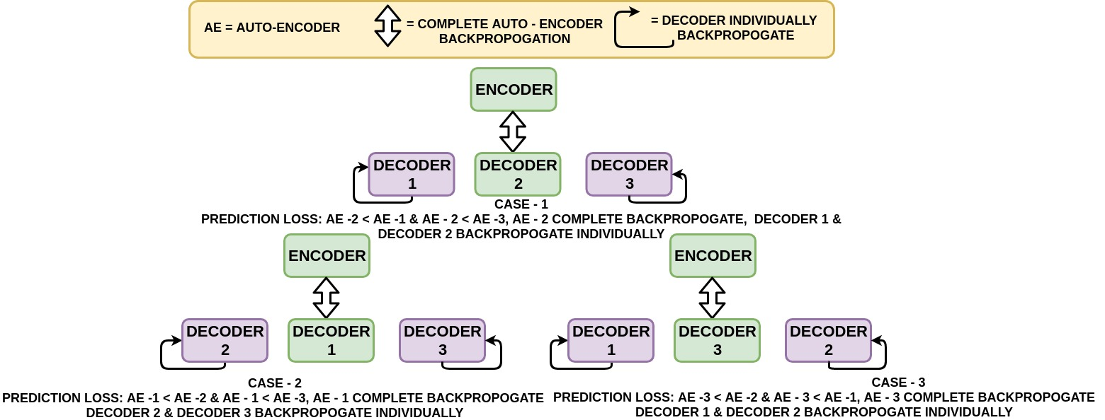
There can be six possible conditions in your network:
loss_1: Autoencoder 1 loss
loss_2: Autoencoder 2 loss
loss_3: Autoencoder 3 loss

if loss_1 < loss_2 and loss_1 < loss_3:
    train_1 = autoencoder_1.train_on_batch(batch_train_X,batch_train_Y)
    myfile_ae1_loss.write("%f \n" % (train_1))
    print ('epoch_num: %d batch_num: %d AE_Train_loss_1: %f\n' % (j,batch,train_1))
    #myfile.write('epoch_num: %d batch_num: %d AE_Train_loss_1: %f\n' % (j,batch,train_1))
    for layer in autoencoder_2.layers[:34]:
        layer.trainable = False
    for layer in autoencoder_3.layers[:34]:
        layer.trainable = False
    #autoencoder_2.summary()
    #autoencoder_3.summary()
    train_2 = autoencoder_2.train_on_batch(batch_train_X,batch_train_Y)
    train_3 = autoencoder_3.train_on_batch(batch_train_X,batch_train_Y)
    myfile_dec2_loss.write("%f \n" % (train_2))
    myfile_dec3_loss.write("%f \n" % (train_3))
    print ('epoch_num: %d batch_num: %d Decoder_Train_loss_2: %f\n' % (j,batch,train_2))
    print ('epoch_num: %d batch_num: %d Decoder_loss_3: %f\n' % (j,batch,train_3))
    #myfile.write('epoch_num: %d batch_num: %d Decoder_Train_loss_2: %f\n' % (j,batch,train_2))
    #myfile.write('epoch_num: %d batch_num: %d Decoder_loss_3: %f\n' % (j,batch,train_3))
elif loss_2 < loss_1 and loss_2 < loss_3:
    train_2 = autoencoder_2.train_on_batch(batch_train_X,batch_train_Y)
    myfile_ae2_loss.write("%f \n" % (train_2))
    print ('epoch_num: %d batch_num: %d AE_Train_loss_2: %f\n' % (j,batch,train_2))
    #myfile.write('epoch_num: %d batch_num: %d AE_Train_loss_2: %f\n' % (j,batch,train_2))
    for layer in autoencoder_1.layers[:34]:
        layer.trainable = False
    for layer in autoencoder_3.layers[:34]:
        layer.trainable = False
    #autoencoder_1.summary()
    #autoencoder_3.summary()
    train_1 = autoencoder_1.train_on_batch(batch_train_X,batch_train_Y)
    train_3 = autoencoder_3.train_on_batch(batch_train_X,batch_train_Y)
    myfile_dec1_loss.write("%f \n" % (train_1))
    myfile_dec3_loss.write("%f \n" % (train_3))
    print ('epoch_num: %d batch_num: %d Decoder_Train_loss_1: %f\n' % (j,batch,train_1))
    print ('epoch_num: %d batch_num: %d Decoder_Train_loss_3: %f\n' % (j,batch,train_3))
    #myfile.write('epoch_num: %d batch_num: %d Decoder_Train_loss_1: %f\n' % (j,batch,train_1))
    #myfile.write('epoch_num: %d batch_num: %d Decoder_Train_loss_3: %f\n' % (j,batch,train_3))
elif loss_3 < loss_1 and loss_3 < loss_2:
    train_3 = autoencoder_3.train_on_batch(batch_train_X,batch_train_Y)
    myfile_ae3_loss.write("%f \n" % (train_3))
    print ('epoch_num: %d batch_num: %d AE_Train_loss_3: %f\n' % (j,batch,train_3))
    #myfile.write('epoch_num: %d batch_num: %d AE_Train_loss_3: %f\n' % (j,batch,train_3))
    for layer in autoencoder_1.layers[:34]:
        layer.trainable = False
    for layer in autoencoder_2.layers[:34]:
        layer.trainable = False
    #autoencoder_1.summary()
    #autoencoder_2.summary()
    train_1 = autoencoder_1.train_on_batch(batch_train_X,batch_train_Y)
    train_2 = autoencoder_2.train_on_batch(batch_train_X,batch_train_Y)
    myfile_dec1_loss.write("%f \n" %(train_1))
    myfile_dec2_loss.write("%f \n" % (train_2))
    print ('epoch_num: %d batch_num: %d Decoder_Train_loss_1: %f\n' % (j,batch,train_1))
    print ('epoch_num: %d batch_num: %d Decoder_Train_loss_2: %f\n' % (j,batch,train_2))
    #myfile.write('epoch_num: %d batch_num: %d Decoder_Train_loss_1: %f\n' % (j,batch,train_1))
    #myfile.write('epoch_num: %d batch_num: %d Decoder_Train_loss_2: %f\n' % (j,batch,train_2))
elif loss_1 == loss_2:
    train_1 = autoencoder_1.train_on_batch(batch_train_X,batch_train_Y)
    myfile_ae1_loss.write("%f \n" % (train_1))
    print ('epoch_num: %d batch_num: %d AE_Train_loss_1_equal_state: %f\n' % (j,batch,train_1))
    #myfile.write('epoch_num: %d batch_num: %d AE_Train_loss_1_equal_state: %f\n' % (j,batch,train_1))
    for layer in autoencoder_3.layers[:34]:
        layer.trainable = False
    for layer in autoencoder_2.layers[:34]:
        layer.trainable = False
    #autoencoder_2.summary()
    #autoencoder_3.summary()
    train_2 = autoencoder_2.train_on_batch(batch_train_X,batch_train_Y)
    train_3 = autoencoder_3.train_on_batch(batch_train_X,batch_train_Y)
    myfile_dec2_loss.write("%f \n" % (train_2))
    myfile_dec3_loss.write("%f \n" % (train_3))
    print ('epoch_num: %d batch_num: %d Decoder_Train_loss_2_equal_state: %f\n' % (j,batch,train_2))
    print ('epoch_num: %d batch_num: %d Decoder_Train_loss_3_equal_state: %f\n' % (j,batch,train_3))
    #myfile.write('epoch_num: %d batch_num: %d Decoder_Train_loss_2_equal_state: %f\n' % (j,batch,train_2))
    #myfile.write('epoch_num: %d batch_num: %d Decoder_Train_loss_3_equal_state: %f\n' % (j,batch,train_3))
elif loss_2 == loss_3:
    train_2 = autoencoder_2.train_on_batch(batch_train_X,batch_train_Y)
    myfile_ae2_loss.write("%f \n" % (train_2))
    print ('epoch_num: %d batch_num: %d AE_Train_loss_2_equal_state: %f\n' % (j,batch,train_2))
    #myfile.write('epoch_num: %d batch_num: %d AE_Train_loss_2_equal_state: %f\n' % (j,batch,train_2))
    for layer in autoencoder_1.layers[:34]:
        layer.trainable = False
    for layer in autoencoder_3.layers[:34]:
        layer.trainable = False

    #autoencoder_2.summary()
    #autoencoder_3.summary()
    train_1 = autoencoder_1.train_on_batch(batch_train_X,batch_train_Y)
    train_3 = autoencoder_3.train_on_batch(batch_train_X,batch_train_Y)
    myfile_dec1_loss.write("%f \n" % (train_1))
    myfile_dec3_loss.write("%f \n" % (train_3))
    print ('epoch_num: %d batch_num: %d Decoder_Train_loss_1_equal_state: %f\n' % (j,batch,train_1))
    print ('epoch_num: %d batch_num: %d Decoder_Train_loss_3_equal_state: %f\n' % (j,batch,train_3))
    #myfile.write('epoch_num: %d batch_num: %d Decoder_Train_loss_1_equal_state: %f\n' % (j,batch,train_1))
    #myfile.write('epoch_num: %d batch_num: %d Decoder_Train_loss_3_equal_state: %f\n' % (j,batch,train_3))
elif loss_3 == loss_1:
    train_1 = autoencoder_1.train_on_batch(batch_train_X,batch_train_Y)
    myfile_ae1_loss.write("%f \n" % (train_1))
    print ('epoch_num: %d batch_num: %d AE_Train_loss_1_equal_state: %f\n' % (j,batch,train_1))
    #myfile.write('epoch_num: %d batch_num: %d AE_Train_loss_1_equal_state: %f\n' % (j,batch,train_1))
    for layer in autoencoder_2.layers[:34]:
        layer.trainable = False
    for layer in autoencoder_3.layers[:34]:
        layer.trainable = False
    #autoencoder_2.summary()
    #autoencoder_3.summary()
    train_2 = autoencoder_2.train_on_batch(batch_train_X,batch_train_Y)
    train_3 = autoencoder_3.train_on_batch(batch_train_X,batch_train_Y)
    myfile_dec2_loss.write("%f \n" % (train_2))
    myfile_dec3_loss.write("%f \n" % (train_3))
    print ('epoch_num: %d batch_num: %d Decoder_Train_loss_2_equal_state: %f\n' % (j,batch,train_2))
    print ('epoch_num: %d batch_num: %d Decoder_Train_loss_3_equal_state: %f\n' % (j,batch,train_3))
    #myfile.write('epoch_num: %d batch_num: %d Decoder_Train_loss_2_equal_state: %f\n' % (j,batch,train_2))
    #myfile.write('epoch_num: %d batch_num: %d Decoder_Train_loss_3_equal_state: %f\n' % (j,batch,train_3))


    myfile_ae1_loss.close()
    myfile_ae2_loss.close()
    myfile_ae3_loss.close()
    myfile_dec1_loss.close()
    myfile_dec2_loss.close()
    myfile_dec3_loss.close()
This is an essential step since you made few layers in the above conditions False, you need to make those layers True, so that all the autoencoder layers can be used for the test_on_batch function and you don't want them to be kept False throughout the training.
for layer in autoencoder_1.layers[:34]:
            layer.trainable = True
for layer in autoencoder_2.layers[:34]:
            layer.trainable = True
for layer in autoencoder_3.layers[:34]:
            layer.trainable = True
You will save weights in three different ways, below are two of those ways. One you will save weights after every 100 epochs, and second, you will save weights after every epoch. Basically, they are overwritten after every epoch.
if jj % 100 ==0:
            autoencoder_1.save_weights("../Model/CROSSVAL1/CROSSVAL1_AE1_" + str(jj)+".h5")
            autoencoder_2.save_weights("../Model/CROSSVAL1/CROSSVAL1_AE2_" + str(jj)+".h5")
            autoencoder_3.save_weights("../Model/CROSSVAL1/CROSSVAL1_AE3_" + str(jj)+".h5")


autoencoder_1.save_weights("../Model/CROSSVAL1/CROSSVAL1_AE1.h5")
autoencoder_2.save_weights("../Model/CROSSVAL1/CROSSVAL1_AE2.h5")
autoencoder_3.save_weights("../Model/CROSSVAL1/CROSSVAL1_AE3.h5")
You will shuffle the validation data first and then use the same 6 possible conditions that may happen as defined above. So whichever condition is True you will test your model using that particular autoencoder.
Then you calculate two metrics MSE and PSNR between decoded_imgs(predicted) and ground truth. Finally, you save them in the text files.
X_test,y_test = shuffle(X_test,y_test)
if loss_1 < loss_2 and loss_1 < loss_3:
    decoded_imgs = autoencoder_1.predict(X_test)
    mse_7T=  np.mean((y_test[:,:,:,0] - decoded_imgs[:,:,:,0]) ** 2)
    check_7T = math.sqrt(mse_7T)
    psnr_7T = 20 * math.log10( 1.0 / check_7T)


    myfile_valid_psnr_7T.write("%f \n" % (psnr_7T))
    myfile_valid_mse_7T.write("%f \n" % (mse_7T))

    #print (check)
elif loss_2 < loss_1 and loss_2 < loss_3:
    decoded_imgs = autoencoder_2.predict(X_test)
    mse_7T=  np.mean((y_test[:,:,:,0] - decoded_imgs[:,:,:,0]) ** 2)
    check_7T = math.sqrt(mse_7T)
    psnr_7T = 20 * math.log10( 1.0 / check_7T)

    myfile_valid_psnr_7T.write("%f \n" % (psnr_7T))
    myfile_valid_mse_7T.write("%f \n" % (mse_7T))

    #print (check)
elif loss_3 < loss_2 and loss_3 < loss_1:
    decoded_imgs = autoencoder_3.predict(X_test)
    mse_7T=  np.mean((y_test[:,:,:,0] - decoded_imgs[:,:,:,0]) ** 2)
    check_7T = math.sqrt(mse_7T)
    psnr_7T = 20 * math.log10( 1.0 / check_7T)

    myfile_valid_psnr_7T.write("%f \n" % (psnr_7T))
    myfile_valid_mse_7T.write("%f \n" % (mse_7T))
    #print (check)

elif loss_1 == loss_2:
    decoded_imgs = autoencoder_1.predict(X_test)
    mse_7T=  np.mean((y_test[:,:,:,0] - decoded_imgs[:,:,:,0]) ** 2)
    check_7T = math.sqrt(mse_7T)
    psnr_7T = 20 * math.log10( 1.0 / check_7T)

    myfile_valid_psnr_7T.write("%f \n" % (psnr_7T))
    myfile_valid_mse_7T.write("%f \n" % (mse_7T))


elif loss_2 == loss_3:
    decoded_imgs = autoencoder_2.predict(X_test)
    mse_7T=  np.mean((y_test[:,:,:,0] - decoded_imgs[:,:,:,0]) ** 2)
    check_7T = math.sqrt(mse_7T)
    psnr_7T = 20 * math.log10( 1.0 / check_7T)

    myfile_valid_psnr_7T.write("%f \n" % (psnr_7T))
    myfile_valid_mse_7T.write("%f \n" % (mse_7T))


elif loss_3 == loss_1:
    decoded_imgs = autoencoder_3.predict(X_test)
    mse_7T=  np.mean((y_test[:,:,:,0] - decoded_imgs[:,:,:,0]) ** 2)
    check_7T = math.sqrt(mse_7T)
    psnr_7T = 20 * math.log10( 1.0 / check_7T)

    myfile_valid_psnr_7T.write("%f \n" % (psnr_7T))
    myfile_valid_mse_7T.write("%f \n" % (mse_7T))
Here you save the weights only when the PSNR between the predicted 7T and ground truth (7T) is the maximum compared to the previous PSNR values stored in the psnr_gray_channel list.
if max(psnr_gray_channel) < psnr_7T:
            autoencoder_1.save_weights("../Model/CROSSVAL1/CROSSVAL1_AE1_" + str(jj)+".h5")
            autoencoder_2.save_weights("../Model/CROSSVAL1/CROSSVAL1_AE2_" + str(jj)+".h5")
            autoencoder_3.save_weights("../Model/CROSSVAL1/CROSSVAL1_AE3_" + str(jj)+".h5")

    psnr_gray_channel.append(psnr_7T)
You will define a numpy matrix temp that has a size of 176 x 528 since there will be 3 images saved in one row each with a dimension of 176 x 176. You will save any one of the images out of all the validation 3T, 7T and predicted and multiplied the matrix by 255 since the images were scaled down between 0 and 1.
Finally using scipy function, you will save the image.
temp = np.zeros([resizeTo,resizeTo*3])
temp[:resizeTo,:resizeTo] = X_test[0,:,:,0]
temp[:resizeTo,resizeTo:resizeTo*2] = y_test[0,:,:,0]
temp[:resizeTo,2*resizeTo:] = decoded_imgs[0,:,:,0]
temp = temp*255
scipy.misc.imsave('../Results/1_encoder_3_decoders_complete_slices_single_channel/' + str(j) + '.jpg', temp)
j +=1
Let's close the PSNR and MSE files at the end.
myfile_valid_psnr_7T.close()
myfile_valid_mse_7T.close()
Finally, at the end, you will reduce the learning rate by 10% of its current value after every 20 epochs.
if jj % 20 ==0:
        learning_rate = learning_rate - learning_rate * 0.10
You'll address the following topics in part-2 of this tutorial:
nibabel.Before you start following along with this tutorial make sure you have the exact same module versions as stated below:
Note: Before you begin, please note that the model will be trained on a system with Nvidia 1080 Ti GPU Xeon e5 GeForce processor with 32GB RAM. If you are using Jupyter Notebook, you will need to add three more lines of code where you specify CUDA device order and CUDA visible devices using a module called os.
In the code below, you basically set environment variables in the notebook using os.environ. It's good to do the following before initializing Keras to limit Keras backend TensorFlow to use the first GPU. If the machine on which you train on has a GPU on 0, make sure to use 0 instead of 1. You can check that by running a simple command on your terminal: for example, nvidia-smi
import os
os.environ["CUDA_DEVICE_ORDER"]="PCI_BUS_ID"
os.environ["CUDA_VISIBLE_DEVICES"]="0" #model will be trained on GPU
First, you import all the required modules like tensorflow, numpy and most importantly keras and the required functions or layers like Input, Conv2D,MaxPooling2D, etc. since you'll be using all these frameworks for training the model!
To read the nifti format images, you also have to import a module called nibabel.
import os
from keras.layers import Input,Dense,Flatten,Dropout,merge,Reshape,Conv2D,MaxPooling2D,UpSampling2D
from keras.layers.normalization import BatchNormalization
from keras.models import Model,Sequential
from keras.callbacks import ModelCheckpoint
from keras.optimizers import Adadelta, RMSprop,SGD,Adam
from keras import regularizers
from keras import backend as K
import numpy as np
import scipy.misc
import numpy.random as rng
from sklearn.utils import shuffle
import nibabel as nib
from sklearn.cross_validation import train_test_split
import math
The brain MRI 3T and 7T dataset consists of 3D volumes each volume has in total 207 slices/images of brain MRI's taken at different slices of the brain. Each slice is of dimension 173 x 173. The images are single channel grayscale images. There are in total 39 subjects, each subject containing the MRI scan of a patient. The image format is not jpeg, png, etc. but rather a nifti format. You will see in a later section on how to read the nifti format images.
The dataset consists of T1 modality MR images, T1 sequences are traditionally considered good for evaluation of anatomic structures. The dataset on which you will be working today consists of 3T and 7T Brain MRI's.
The dataset is public and is available for download at this source.
Let's first define the dimensions of the data. You will resize the image dimension from 173x173 to 176x176 in the data reading part. Here we also define the data directory, batch size we use for training the model, a number of channels, an Input() layer,train and test matrices as a list and finally for rescaling we load the text file which has the minimum and maximum values of the MRI dataset.
x,y = 173,173
full_z = 207
resizeTo=176
inChannel = outChannel = 1
input_shape=(x,y,inChannel)
input_img = Input(shape = (resizeTo, resizeTo, inChannel))
train_matrix = []
test_matrix = []
ff = os.listdir("../test_crossval1")
save = "../Result_nii_crossval1"
folder_ground = os.listdir("../test_g_crossval1")
ToPredict_images=[]
predict_matrix=[]
ground_images=[]
ground_matrix=[]
min_max=np.loadtxt('../maxANDmin.txt')
Next, we load the mri data using the nibabel library and resize the images from 173 x 173 to 176 x 176 by padding zeros in x and y dimension.
Note that when you load a Nifti format volume, Nibabel does not load the image array. It waits until you ask for the array data. The standard way to ask for the array data is to call the get_data() method.
Since you want the 2D slices instead of 3D, you will use the train and test lists that you initialized before; every time you read a volume, you will iterate over all the complete 207 slices of the 3D volume and append each slice one by one into a list.
for f in ff:
    temp = np.zeros([resizeTo,full_z,resizeTo])
    a = nib.load("../test_crossval1" + f)
    affine = a.affine
    a = a.get_data()
    temp[3:,:,3:] = a
    a = temp
    for j in range(full_z):
        predict_matrix.append(a[:,j,:])
for f in ff:
    temp = np.zeros([resizeTo,full_z,resizeTo])
    a = nib.load("../test_g_crossval1" + f)
    affine = a.affine
    a = a.get_data()
    temp[3:,:,3:] = a
    a = temp
    for j in range(full_z):
        ground_matrix.append(a[:,j,:])
Since 3t and 7T test matrices is a list, you will use numpy module to convert the list into a numpy array.
Further, you will convert the type of the numpy array as float32 and also rescale both the input and the ground truth.
ToPredict_images = np.asarray(predict_matrix)
ToPredict_images = ToPredict_images.astype('float32')
mx = min_max[0]
mn = min_max[1]
ToPredict_images[:,:,:,0] = (ToPredict_images[:,:,:,0] - mn ) / (mx - mn)
ground_images = np.asarray(ground_matrix)
ground_images = ground_images.astype('float32')
ground_images[:,:,:,0] = (ground_images[:,:,:,0] - mn ) / (mx - mn)
Next, you will create two new variables ToPredict_images(3T Test/input) and ground_images (7T Test/ground truth) of the shape train and test matrix. This will be a 4D matrix in which the first dimension will be the total number of images, second and third being the dimension of each image and last dimension being the number of channels which is one in this case."
ToPredict_images=np.zeros(shape=[(ToPredict_images.shape[0]),(ToPredict_images.shape[1]),(ToPredict_images.shape[2]),(1)])
ground_images=np.zeros(shape=[(ground_images.shape[0]),(ground_images.shape[1]),(ground_images.shape[2]),(1)])
Then you will iterate over all the images one by one, each time you will reshape the train and test matrix to 176 x 176 and append it to ToPredict_images(3T Test/input) and ground_images (7T Test/ground truth) respectively.
for i in range(ToPredict_images.shape[0]):
    ToPredict_images[i,:,:,0] = ToPredict_images[i,:,:].reshape(resizeTo,resizeTo)
for i in range(ground_images.shape[0]):
    ground_images[i,:,:,0] = ground_images[i,:,:].reshape(resizeTo,resizeTo)
def encoder(input_img):
    conv1 = Conv2D(32, (3, 3), activation='relu', padding='same')(input_img)
    conv1 = BatchNormalization()(conv1)
    conv1 = Conv2D(32, (3,3), activation='relu', padding='same')(conv1)
    conv1 = BatchNormalization()(conv1)
    conv1 = Conv2D(32, (3,3), activation='relu', padding='same')(conv1)
    conv1 = BatchNormalization()(conv1)
    pool1 = MaxPooling2D(pool_size=(2, 2))(conv1)
    conv2 = Conv2D(64, (3, 3), activation='relu', padding='same')(pool1)
    conv2 = BatchNormalization()(conv2)
    conv2 = Conv2D(64, (3, 3), activation='relu', padding='same')(conv2)
    conv2 = BatchNormalization()(conv2)
    conv2 = Conv2D(64, (3, 3), activation='relu', padding='same')(conv2)
    conv2 = BatchNormalization()(conv2)
    pool2 = MaxPooling2D(pool_size=(2, 2))(conv2)
    conv3 = Conv2D(128, (3, 3), activation='relu', padding='same')(pool2)
    conv3 = BatchNormalization()(conv3)
    conv3 = Conv2D(128, (3, 3), activation='relu', padding='same')(conv3)
    conv3 = BatchNormalization()(conv3)
    conv3 = Conv2D(128, (3, 3), activation='relu', padding='same')(conv3)
    conv3 = BatchNormalization()(conv3)
    pool3 = MaxPooling2D(pool_size=(2, 2))(conv3)
    conv4 = Conv2D(256, (3, 3), activation='relu', padding='same')(pool3)
    conv4 = BatchNormalization()(conv4)
    conv4 = Conv2D(256, (3, 3), activation='relu', padding='same')(conv4)
    conv4 = BatchNormalization()(conv4)
    conv4 = Conv2D(256, (3, 3), activation='relu', padding='same')(conv4)
    conv4 = BatchNormalization()(conv4)
    conv5 = Conv2D(512, (3, 3), activation='relu', padding='same')(conv4)
    conv5 = BatchNormalization()(conv5)
    conv5 = Conv2D(512, (3, 3), activation='relu', padding='same')(conv5)
    conv5 = BatchNormalization()(conv5)
    conv5 = Conv2D(512, (3, 3), activation='sigmoid', padding='same')(conv5)
    conv5 = BatchNormalization()(conv5)
    return conv5,conv4,conv3,conv2,conv1
def decoder(conv5,conv4,conv3,conv2,conv1):
    up6 = merge([conv5, conv4], mode='concat', concat_axis=3)
    conv6 = Conv2D(256, (3, 3), activation='relu', padding='same')(up6)
    conv6 = BatchNormalization()(conv6)
    conv6 = Conv2D(256, (3, 3), activation='relu', padding='same')(conv6)
    conv6 = BatchNormalization()(conv6)
    conv6 = Conv2D(256, (3, 3), activation='relu', padding='same')(conv6)
    conv6 = BatchNormalization()(conv6)
    up7 = UpSampling2D((2,2))(conv6)
    up7 = merge([up7, conv3], mode='concat', concat_axis=3)
    conv7 = Conv2D(128, (3, 3), activation='relu', padding='same')(up7)
    conv7 = BatchNormalization()(conv7)
    conv7 = Conv2D(128, (3, 3), activation='relu', padding='same')(conv7)
    conv7 = BatchNormalization()(conv7)
    conv7 = Conv2D(128, (3, 3), activation='relu', padding='same')(conv7)
    conv7 = BatchNormalization()(conv7)
    up8 = UpSampling2D((2,2))(conv7)
    up8 = merge([up8, conv2], mode='concat', concat_axis=3)
    conv8 = Conv2D(64, (3, 3), activation='relu', padding='same')(up8)
    conv8 = BatchNormalization()(conv8)
    conv8 = Conv2D(64, (3, 3), activation='relu', padding='same')(conv8)
    conv8 = BatchNormalization()(conv8)
    conv8 = Conv2D(64, (3, 3), activation='relu', padding='same')(conv8)
    conv8 = BatchNormalization()(conv8)
    up9 = UpSampling2D((2,2))(conv8)
    up9 = merge([up9, conv1], mode='concat', concat_axis=3)
    conv9 = Conv2D(32, (3, 3), activation='relu', padding='same')(up9)
    conv9 = BatchNormalization()(conv9)
    conv9 = Conv2D(32, (3, 3), activation='relu', padding='same')(conv9)
    conv9 = BatchNormalization()(conv9)
    conv9 = Conv2D(32, (3, 3), activation='relu', padding='same')(conv9)
    conv9 = BatchNormalization()(conv9)
    decoded = Conv2D(1, (3, 3), activation='sigmoid', padding='same')(conv9)
    return decoded
Next, you will employ a mean square error in which you'll exclude the values(pixels) of both the ground truth y_t and y_p that are equal to zero.
def root_mean_sq_GxGy(y_t, y_p):
    a1=1
    zero = tf.constant(0, dtype=tf.float32)
    where = tf.not_equal(y_t, zero)
    a_t=tf.boolean_mask(y_t,where,name='boolean_mask')
    a_p=tf.boolean_mask(y_p,where,name='boolean_mask')
    return a1*(K.sqrt(K.mean((K.square(a_t-a_p)))))
First, let's call the encoder function by passing in the input to it. Since you are using the merge connection in your architecture, the encoder function will return the output of five convolution layers which you then merge with all three decoders output separately.
conv5,conv4,conv3,conv2,conv1 = encoder(input_img)
Now let's create three different models and load the three trained model weights into them.
autoencoder_1 = Model(input_img, decoder(conv5,conv4,conv3,conv2,conv1))

autoencoder_1.load_weights("../Model/CROSSVAL1/CROSSVAL1_AE1.h5")
autoencoder_2 = Model(input_img, decoder(conv5,conv4,conv3,conv2,conv1))

autoencoder_2.load_weights("../Model/CROSSVAL1/CROSSVAL1_AE2.h5")
autoencoder_3 = Model(input_img, decoder(conv5,conv4,conv3,conv2,conv1))

autoencoder_3.load_weights("../Model/CROSSVAL1/CROSSVAL1_AE3.h5")
Let's quickly initialize two numpy arrays each of size 11 x 3 x 1 where the first dimension will represent the number of volumes you will use for testing your model. The second dimension will represent the MSE and PSNR between: Predicted Output 7T MR images and Ground Truth 7T MR images, Predicted Output and Input 3T MR images, Input 3T MR images and Ground Truth 7T MR images; the third dimension will represent the number of channels that you will input to your model!
mse= np.zeros([11,3,1])
psnr= np.zeros([11,3,1])
i=0 #for iterating over the slices of all the 11 volumes
In the next part of the cell, you will iterate over all 11 volumes one by one. In each iteration, you will predict each volume using all the three autoencoders and finally average out the predictions.
In each volume, you will be iterating over the number of channels of that volume and calculate PSNR and MSE for three different cases as discussed above.
Then using the nibabel library, you will save the predicted output, input (3T) and ground truth (7T) as .nii format files: each of the 11 volumes comprising of 207 slices.
Finally, you will save the PSNR matrix in a text file using the numpy library.
As stated in the paper averaging the predicted outputs helps in reducing noise effects but preserves the local features in the reconstructed images, due to which the PSNR improves over the individual decoder outputs.
for j in range(11):
    decoded_imgs_1 = autoencoder_1.predict(ToPredict_images[i:i+207,:,:,:])
    decoded_imgs_2 = autoencoder_2.predict(ToPredict_images[i:i+207,:,:,:])
    decoded_imgs_3 = autoencoder_3.predict(ToPredict_images[i:i+207,:,:,:])
    decoded_imgs = np.mean( np.array([ decoded_imgs_1, decoded_imgs_2,decoded_imgs_3 ]), axis=0 )
    for channel in range(1):
        mse[j,0,channel]=  np.mean((ground_images[i:i+207,:,:,channel] - decoded_imgs[:,:,:,channel]) ** 2)
        psnr[j,0,channel] = 20 * math.log10( 1.0 / math.sqrt(mse[j,0,channel]))
        mse[j,1,channel]=  np.mean((ground_images[i:i+207,:,:,channel] - ToPredict_images[i:i+207,:,:,channel])** 2)
        psnr[j,1,channel] = 20 * math.log10( 1.0 / math.sqrt(mse[j,1,channel]))
        mse[j,2,channel] =  np.mean((ToPredict_images[i:i+207,:,:,channel] - decoded_imgs[:,:,:,channel]) ** 2)
        checklt = math.sqrt(mse[j,2,channel])
        psnr[j,2,channel] = 20 * math.log10( 1.0 / math.sqrt(mse[j,2,channel]))
    obj = nib.Nifti1Image(decoded_imgs, affine)
    string =str(j)+'_crossval1.nii'
    nib.save(obj, save + string)
    obj = nib.Nifti1Image(ground_images[i:i+207,:,:,:], affine)
    string =str(j)+'_ground_images_crossval1.nii'
    nib.save(obj, save + string)
    obj = nib.Nifti1Image(ToPredict_images[i:i+207,:,:,:], affine)
    string =str(j)+'_ToPredict_images_crossval1.nii'
    nib.save(obj, save + string)
    i=i+207


np.savetxt('psnr_all_slices.txt',psnr[:,:,0])
If you would like to learn more about Python, take DataCamp's Introduction to Data Visualization with Matplotlib course.
Check out the Keras Tutorial: Deep Learning in Python.
Learn more about Python and Deep Learning
Course
Course
Course
Tutorial
Karlijn Willems
Tutorial
Aditya Sharma
Tutorial
Aditya Sharma
Tutorial
Aditya Sharma
Tutorial
Aditya Sharma
Tutorial
Aditya Sharma