Autoencoder as a Classifier using Fashion-MNIST Dataset Tutorial

Note: This tutorial will mostly cover the practical implementation of classification using the convolutional neural network and convolutional autoencoder. So, if you are not yet aware of the convolutional neural network (CNN) and autoencoder, you might want to look at CNN and Autoencoder tutorial.

More specifically, you'll tackle the following topics in today's tutorial:

• In the beginning you will be briefed about the Fashion-MNIST Data. You'll use Python's various libraries to load, explore and analyze your data,
• After that, you'll preprocess your data: you'll learn how to resize, rescale the data, verify the data types of the images and split up your data in training and validation sets.
• With all of this done, you can construct the convolutional autoencoder model: you'll learn how to model the data and form the network. Next, you'll compile, train the model, visualizing the accuracy and loss plots and finally save the model.
• Next, you will segment your fashion-mnist data: you'll first convert your labels into one-hot encoding vectors, split up your training and validation images along with their respective labels. Then you'll define the same encoder function that you will use in autoencoder architecture followed by fully connected layers.
• You'll learn how to load the weights of a trained model in to few layers of the new model, verify the weight matrices of trained and new model, make few layers of the new model false, and finally you'll compile the new classification model, train the model and save the weights.
• You will re-train the model with all layers trainable, evaluate the model, visualizing the accuracy and loss plots, make predictions on the test data, convert the probabilities into class labels and plot few test samples that your model correctly classified and incorrectly classified.
• Finally, you will visualize the classification report which will give you more in-depth intuition about which class was (in)correctly classified by your model.

The Fashion-MNIST Data Set

Before we begin loading the dataset and start processing it, it is a better idea to have a brief intuition about what kind of dataset it is, what is the dimension of the data and how many different classes are in the dataset.

Fashion-MNIST dataset is a 28x28 grayscale images of 70,000 fashion products from 10 categories, with 7,000 images per category. The training set has 60,000 images, and the test set has 10,000 images. Fashion-MNIST is a replacement for the original MNIST dataset for producing better results, the image dimensions, training and test splits are similar to the original MNIST dataset. The dataset is freely available on this URL and can be loaded using both tensorflow and keras as a framework without having to download it on your computer.

Similar to MNIST the Fashion-MNIST also consists of 10 classes, but instead of handwritten digits, we have 10 different classes of fashion accessories like sandals, shirt, trousers, etc.

The task at hand is to train a convolutional autoencoder and use the encoder part of the autoencoder combined with fully connected layers to recognize a new sample from the test set correctly.

Tip: if you want to learn how to implement a Multi-Layer Perceptron (MLP) for classification tasks with the MNIST dataset, check out this tutorial.

In the code below, you basically set environment variables in the notebook using os.environ. It's good to do the following before initializing Keras to limit Keras backend TensorFlow to use the first GPU. If the machine on which you train on has a GPU on 0, make sure to use 0 instead of 1. You can check that by running a simple command on your terminal: for example, nvidia-smi

import os
os.environ["CUDA_DEVICE_ORDER"]="PCI_BUS_ID"
os.environ["CUDA_VISIBLE_DEVICES"]="0" #model will be trained on GPU 0

Loading in the Data

Next, you import all the required modules like numpy, matplotlib and most importantly Keras, since in today's tutorial you will be using keras as the framework!

import keras
from matplotlib import pyplot as plt
import numpy as np
import gzip
%matplotlib inline
from keras.models import Model
from keras.optimizers import RMSprop
from keras.layers import Input,Dense,Flatten,Dropout,merge,Reshape,Conv2D,MaxPooling2D,UpSampling2D,Conv2DTranspose
from keras.layers.normalization import BatchNormalization
from keras.models import Model,Sequential
from keras.callbacks import ModelCheckpoint
from keras.optimizers import Adadelta, RMSprop,SGD,Adam
from keras import regularizers
from keras import backend as K
from keras.utils import to_categorical

Using TensorFlow backend.
/usr/local/lib/python2.7/dist-packages/h5py/__init__.py:34: FutureWarning: Conversion of the second argument of issubdtype from `float` to `np.floating` is deprecated. In future, it will be treated as `np.float64 == np.dtype(float).type`.
  from ._conv import register_converters as _register_converters

Here, you define a function that opens the gzip file, reads the file using bytestream.read(). You pass the image dimension and the number of images you have in total to this function. Then, using np.frombuffer(), you convert the string stored in variable buf into a NumPy array of type float32.

Once it is converted into a NumPy array, you reshape the array into a three-dimensional array or tensor where the first dimension is a number of images, and the second and third dimension being the dimension of the image. Finally, you return the NumPy array data.

def extract_data(filename, num_images):
    with gzip.open(filename) as bytestream:
        bytestream.read(16)
        buf = bytestream.read(28 * 28 * num_images)
        data = np.frombuffer(buf, dtype=np.uint8).astype(np.float32)
        data = data.reshape(num_images, 28,28)
        return data

You will now call the function extract_data() by passing the training and testing files along with their corresponding number of images.

train_data = extract_data('train-images-idx3-ubyte.gz', 60000)
test_data = extract_data('t10k-images-idx3-ubyte.gz', 10000)

Similarly, you define an extract labels function that opens the gzip file, reads the file using bytestream.read(), to which you pass the label dimension (1) and the number of images you have in total. Then, using np.frombuffer(), you convert the string stored in variable buf into a NumPy array of type int64.

This time, you do not need to reshape the array since the variable labels will return a column vector of dimension 60,000 x 1. Finally, you return the NumPy array labels.

def extract_labels(filename, num_images):
    with gzip.open(filename) as bytestream:
        bytestream.read(8)
        buf = bytestream.read(1 * num_images)
        labels = np.frombuffer(buf, dtype=np.uint8).astype(np.int64)
        return labels

You will now call the function extract label by passing the training and testing label files along with their corresponding number of images.

train_labels = extract_labels('train-labels-idx1-ubyte.gz',60000)
test_labels = extract_labels('t10k-labels-idx1-ubyte.gz',10000)

Once you have the training and testing data loaded, you are all set to analyze the data in order to get some intuition about the dataset that you are going to work with for today's tutorial!

Data Exploration

Let's now analyze how images in the dataset look like and also see the dimension of the images with the help of the NumPy array attribute .shape:

# Shapes of training set
print("Training set (images) shape: {shape}".format(shape=train_data.shape))

# Shapes of test set
print("Test set (images) shape: {shape}".format(shape=test_data.shape))

Training set (images) shape: (60000, 28, 28)
Test set (images) shape: (10000, 28, 28)

From the above output, you can see that the training data has a shape of 60000 x 28 x 28 since there are 60,000 training samples each of 28 x 28 dimensional matrix. Similarly, the test data has a shape of 10000 x 28 x 28 since there are 10,000 testing samples.

Note that in the task of reconstructing using convolutional autoencoder you won't need training and testing labels. Your training images will both act as the input as well as the ground truth similar to the labels you have in classification task.

But for the classification task you will also need your labels along with the images which you will be doing later on in the tutorial. Even though the task at hand will only be dealing with the training and testing images. However, for exploration purposes, which might give you a better intuition about the data, you'll make use of the labels.

Let's create a dictionary that will have class names with their corresponding categorical class labels:

# Create dictionary of target classes
label_dict = {
 0: 'A',
 1: 'B',
 2: 'C',
 3: 'D',
 4: 'E',
 5: 'F',
 6: 'G',
 7: 'H',
 8: 'I',
 9: 'J',
}

Now, let's take a look at a couple of the images in your dataset:

plt.figure(figsize=[5,5])

# Display the first image in training data
plt.subplot(121)
curr_img = np.reshape(train_data[10], (28,28))
curr_lbl = train_labels[10]
plt.imshow(curr_img, cmap='gray')
plt.title("(Label: " + str(label_dict[curr_lbl]) + ")")

# Display the first image in testing data
plt.subplot(122)
curr_img = np.reshape(test_data[10], (28,28))
curr_lbl = test_labels[10]
plt.imshow(curr_img, cmap='gray')
plt.title("(Label: " + str(label_dict[curr_lbl]) + ")")

Text(0.5,1,'(Label: E)')

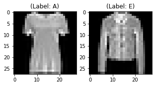
The output of the above two plots is one of the sample images from both training and testing data, and these images are assigned a class label of 0 or A, on the one hand, and 4 or E, on the other hand. Similarly, other alphabets will have different labels, but similar alphabets will have the same labels. This means that all the 6,000 class E images will have a class label of 4.

Data Preprocessing

The images of the dataset are indeed grayscale images with pixel values ranging from 0 to 255 with a dimension of 28 x 28, so before we feed the data into the model, it is very important to preprocess it. You'll first convert each 28 x 28 image of train and test set into a matrix of size 28 x 28 x 1, which you can feed into the network:

train_data = train_data.reshape(-1, 28,28, 1)
test_data = test_data.reshape(-1, 28,28, 1)
train_data.shape, test_data.shape

((60000, 28, 28, 1), (10000, 28, 28, 1))

Next, you want to make sure to check the data type of the training and testing NumPy arrays, it should be in float32 format, if not you will need to convert it into this format, but since you already have converted it while reading the data, you no longer need to do this again. You also have to rescale the pixel values in range 0 - 1 inclusive. So let's do that!

Don't forget to verify the training and testing data types:

train_data.dtype, test_data.dtype

(dtype('float32'), dtype('float32'))

Next, rescale the training and testing data with the maximum pixel value of the training and testing data:

np.max(train_data), np.max(test_data)

(255.0, 255.0)

train_data = train_data / np.max(train_data)
test_data = test_data / np.max(test_data)

Let's verify the maximum value of training and testing data which should be 1.0 after rescaling it!

np.max(train_data), np.max(test_data)

(1.0, 1.0)

After all of this, it's important to partition the data. In order for our model to generalize well, you split the training data into two parts: a training and a validation set. You will train your model on 80% of the data and validate it on 20% of the remaining training data.

This will also help you in reducing the chances of overfitting, as you will be validating your model on data it would not have seen in the training phase.

You can use the train_test_split module of scikit-learn to divide the data properly:

from sklearn.model_selection import train_test_split
train_X,valid_X,train_ground,valid_ground = train_test_split(train_data,
                                                             train_data,
                                                             test_size=0.2,
                                                             random_state=13)

Note: You will be using the above data splitting twice, once for the task of reconstructing using convolutional autoencoder for which you don't need training and testing labels. That's why you will pass the training images twice. Your training images will both act as the input as well as the ground truth similar to the labels you have in the classification task.

But for the classification task, you will also pass your labels along with the images which you will be doing later on in the tutorial.

Now you are all set to define the network and feed the data into the network. So without any further ado, let's jump to the next step!

The Convolutional Autoencoder

The images are of size 28 x 28 x 1 or a 30976-dimensional vector. You convert the image matrix to an array, rescale it between 0 and 1, reshape it so that it's of size 28 x 28 x 1, and feed this as an input to the network.

Also, you will use a batch size of 128 using a higher batch size of 256 or 512 is also preferable it all depends on the system you train your model. It contributes heavily in determining the learning parameters and affects the prediction accuracy.

batch_size = 64
epochs = 200
inChannel = 1
x, y = 28, 28
input_img = Input(shape = (x, y, inChannel))
num_classes = 10

As you might already know well before, the autoencoder is divided into two parts: there's an encoder and a decoder.

Encoder: It has 4 Convolution blocks, each block has a convolution layer followed by a batch normalization layer. Max-pooling layer is used after the first and second convolution blocks.

• The first convolution block will have 32 filters of size 3 x 3, followed by a downsampling (max-pooling) layer,
• The second block will have 64 filters of size 3 x 3, followed by another downsampling layer,
• The third block of encoder will have 128 filters of size 3 x 3,
• The fourth block of encoder will have 256 filters of size 3 x 3.

Decoder: It has 3 Convolution blocks, each block has a convolution layer followed by a batch normalization layer. Upsampling layer is used after the second and third convolution blocks.

• The first block will have 128 filters of size 3 x 3,
• The second block will have 64 filters of size 3 x 3 followed by another upsampling layer,
• The third block will have 32 filters of size 3 x 3 followed by another upsampling layer,
• The final layer of encoder will have 1 filter of size 3 x 3 which will reconstruct back the input having a single channel.

The max-pooling layer will downsample the input by two times each time you use it, while the upsampling layer will upsample the input by two times each time it is used.

Note: The number of filters, the filter size, the number of layers, number of epochs you train your model, are all hyperparameters and should be decided based on your own intuition, you are free to try new experiments by tweaking with these hyperparameters and measure the performance of your model. And that is how you will slowly learn the art of deep learning!

Let's create separate encoder and decoder functions since you will be using encoder weights later on for classification purpose!

def encoder(input_img):
    #encoder
    #input = 28 x 28 x 1 (wide and thin)
    conv1 = Conv2D(32, (3, 3), activation='relu', padding='same')(input_img) #28 x 28 x 32
    conv1 = BatchNormalization()(conv1)
    conv1 = Conv2D(32, (3, 3), activation='relu', padding='same')(conv1)
    conv1 = BatchNormalization()(conv1)
    pool1 = MaxPooling2D(pool_size=(2, 2))(conv1) #14 x 14 x 32
    conv2 = Conv2D(64, (3, 3), activation='relu', padding='same')(pool1) #14 x 14 x 64
    conv2 = BatchNormalization()(conv2)
    conv2 = Conv2D(64, (3, 3), activation='relu', padding='same')(conv2)
    conv2 = BatchNormalization()(conv2)
    pool2 = MaxPooling2D(pool_size=(2, 2))(conv2) #7 x 7 x 64
    conv3 = Conv2D(128, (3, 3), activation='relu', padding='same')(pool2) #7 x 7 x 128 (small and thick)
    conv3 = BatchNormalization()(conv3)
    conv3 = Conv2D(128, (3, 3), activation='relu', padding='same')(conv3)
    conv3 = BatchNormalization()(conv3)
    conv4 = Conv2D(256, (3, 3), activation='relu', padding='same')(conv3) #7 x 7 x 256 (small and thick)
    conv4 = BatchNormalization()(conv4)
    conv4 = Conv2D(256, (3, 3), activation='relu', padding='same')(conv4)
    conv4 = BatchNormalization()(conv4)
    return conv4

def decoder(conv4):    
    #decoder
    conv5 = Conv2D(128, (3, 3), activation='relu', padding='same')(conv4) #7 x 7 x 128
    conv5 = BatchNormalization()(conv5)
    conv5 = Conv2D(128, (3, 3), activation='relu', padding='same')(conv5)
    conv5 = BatchNormalization()(conv5)
    conv6 = Conv2D(64, (3, 3), activation='relu', padding='same')(conv5) #7 x 7 x 64
    conv6 = BatchNormalization()(conv6)
    conv6 = Conv2D(64, (3, 3), activation='relu', padding='same')(conv6)
    conv6 = BatchNormalization()(conv6)
    up1 = UpSampling2D((2,2))(conv6) #14 x 14 x 64
    conv7 = Conv2D(32, (3, 3), activation='relu', padding='same')(up1) # 14 x 14 x 32
    conv7 = BatchNormalization()(conv7)
    conv7 = Conv2D(32, (3, 3), activation='relu', padding='same')(conv7)
    conv7 = BatchNormalization()(conv7)
    up2 = UpSampling2D((2,2))(conv7) # 28 x 28 x 32
    decoded = Conv2D(1, (3, 3), activation='sigmoid', padding='same')(up2) # 28 x 28 x 1
    return decoded

After the model is created, you have to compile it using the optimizer to be RMSProp.

Note that you also have to specify the loss type via the argument loss. In this case, that's the mean squared error, since the loss after every batch will be computed between the batch of predicted output and the ground truth using mean squared error pixel by pixel:

autoencoder = Model(input_img, decoder(encoder(input_img)))
autoencoder.compile(loss='mean_squared_error', optimizer = RMSprop())

Let's visualize the layers that you created in the above step by using the summary function. This will show a number of parameters (weights and biases) in each layer and also the total parameters in your model.

autoencoder.summary()

_________________________________________________________________
Layer (type)                 Output Shape              Param #   
=================================================================
input_2 (InputLayer)         (None, 28, 28, 1)         0         
_________________________________________________________________
conv2d_16 (Conv2D)           (None, 28, 28, 32)        320       
_________________________________________________________________
batch_normalization_15 (Batc (None, 28, 28, 32)        128       
_________________________________________________________________
...

batch_normalization_28 (Batc (None, 14, 14, 32)        128       
_________________________________________________________________
up_sampling2d_4 (UpSampling2 (None, 28, 28, 32)        0         
_________________________________________________________________
conv2d_30 (Conv2D)           (None, 28, 28, 1)         289       
=================================================================
Total params: 1,758,657
Trainable params: 1,755,841
Non-trainable params: 2,816
_________________________________________________________________

It's finally time to train the model with Keras' fit() function! The model trains for 200 epochs. The fit() function will return a history object; By storing the result of this function in autoencoder_train, you can use it later to plot the loss function plot between training and validation which will help you to analyze your model's performance visually.

Train the Model

autoencoder_train = autoencoder.fit(train_X, train_ground, batch_size=batch_size,epochs=epochs,verbose=1,validation_data=(valid_X, valid_ground))

Train on 48000 samples, validate on 12000 samples
Epoch 1/200
48000/48000 [==============================] - 19s - loss: 0.0202 - val_loss: 0.0114s: 0.020
Epoch 2/200
48000/48000 [==============================] - 17s - loss: 0.0087 - val_loss: 0.0071  
...  
Epoch 199/200
48000/48000 [==============================] - 18s - loss: 7.0886e-04 - val_loss: 8.9876e-04
Epoch 200/200
48000/48000 [==============================] - 18s - loss: 7.0929e-04 - val_loss: 0.0010

Finally! You trained the model on the fashion-mnist dataset for 100 epochs, Now, let's plot the loss plot between training and validation data to visualize the model performance.

loss = autoencoder_train.history['loss']
val_loss = autoencoder_train.history['val_loss']
epochs = range(200)
plt.figure()
plt.plot(epochs, loss, 'bo', label='Training loss')
plt.plot(epochs, val_loss, 'b', label='Validation loss')
plt.title('Training and validation loss')
plt.legend()
plt.show()

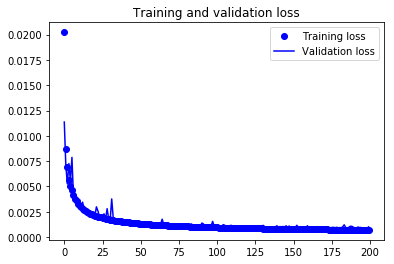
Finally, you can see that the validation loss and the training loss both are in sync. It shows that your model is not overfitting: the validation loss is decreasing and not increasing, and there is rarely any gap between training and validation loss throughout the training phase.

Therefore, you can say that your model's generalization capability is good.

But remember the task at hand is to use the above-trained model's encoder part to classify the fashion mnist images. So, let's move to the next part now!

Save the Model

Since you will need the encoder weights in your classification task, first let's save the complete autoencoder weights. You will learn how you can extract the encoder weights soon.

autoencoder.save_weights('autoencoder.h5')

Segmenting the Fashion Mnist Images

Now you will be using the trained autoencoder's head, i.e., the encoder part and will be loading the weights of the autoencoder you just now trained but only in the encoder part of the model.

You will add a few dense or fully connected layers to the encoder to classify fashion mnist images.

• Let's first convert the labels into one-hot encoding vectors.
  
  For those of you who do not know about one-hot encoding:

In one-hot encoding, you convert the categorical data into a vector of numbers. The reason why you convert the categorical data in one hot encoding is that machine learning algorithms cannot work with categorical data directly. You generate one boolean column for each category or class. Only one of these columns could take on the value 1 for each sample. Hence, the term one-hot encoding.

For your problem statement, the one hot encoding will be a row vector, and for each image, it will have a dimension of 1 x 10. The important thing to note here is that the vector consists of all zeros except for the class that it represents, and for that, it is 1.

So let's convert the labels into one-hot encoding vectors:

# Change the labels from categorical to one-hot encoding
train_Y_one_hot = to_categorical(train_labels)
test_Y_one_hot = to_categorical(test_labels)

# Display the change for category label using one-hot encoding
print('Original label:', train_labels[0])
print('After conversion to one-hot:', train_Y_one_hot[0])

('Original label:', 9)
('After conversion to one-hot:', array([0., 0., 0., 0., 0., 0., 0., 0., 0., 1.]))

That's pretty clear, right?

• This last step is a crucial one which you all have done before as well which is splitting the data into training and validation in the autoencoder training phase. So let's quickly do that step for classification as well. Note that you will use the same random state that you used before and also this time you will pass your labels as well that you just now converted into a one-hot encoding vector.

train_X,valid_X,train_label,valid_label = train_test_split(train_data,train_Y_one_hot,test_size=0.2,random_state=13)

For one last time let's check the shape of training and validation set.

train_X.shape,valid_X.shape,train_label.shape,valid_label.shape

((48000, 28, 28, 1), (12000, 28, 28, 1), (48000, 10), (12000, 10))

Now, let's define the classification model. Remember that you will be using the exact same encoder part as you used in the autoencoder architecture.

def encoder(input_img):
    #encoder
    #input = 28 x 28 x 1 (wide and thin)
    conv1 = Conv2D(32, (3, 3), activation='relu', padding='same')(input_img) #28 x 28 x 32
    conv1 = BatchNormalization()(conv1)
    conv1 = Conv2D(32, (3, 3), activation='relu', padding='same')(conv1)
    conv1 = BatchNormalization()(conv1)
    pool1 = MaxPooling2D(pool_size=(2, 2))(conv1) #14 x 14 x 32
    conv2 = Conv2D(64, (3, 3), activation='relu', padding='same')(pool1) #14 x 14 x 64
    conv2 = BatchNormalization()(conv2)
    conv2 = Conv2D(64, (3, 3), activation='relu', padding='same')(conv2)
    conv2 = BatchNormalization()(conv2)
    pool2 = MaxPooling2D(pool_size=(2, 2))(conv2) #7 x 7 x 64
    conv3 = Conv2D(128, (3, 3), activation='relu', padding='same')(pool2) #7 x 7 x 128 (small and thick)
    conv3 = BatchNormalization()(conv3)
    conv3 = Conv2D(128, (3, 3), activation='relu', padding='same')(conv3)
    conv3 = BatchNormalization()(conv3)
    conv4 = Conv2D(256, (3, 3), activation='relu', padding='same')(conv3) #7 x 7 x 256 (small and thick)
    conv4 = BatchNormalization()(conv4)
    conv4 = Conv2D(256, (3, 3), activation='relu', padding='same')(conv4)
    conv4 = BatchNormalization()(conv4)
    return conv4

Let's define the fully connected layers that you will be stacking up with the encoder function.

def fc(enco):
    flat = Flatten()(enco)
    den = Dense(128, activation='relu')(flat)
    out = Dense(num_classes, activation='softmax')(den)
    return out

encode = encoder(input_img)
full_model = Model(input_img,fc(encode))

for l1,l2 in zip(full_model.layers[:19],autoencoder.layers[0:19]):
    l1.set_weights(l2.get_weights())

Note: The next step is pretty important. In order to be sure whether the weights of the encoder part of the autoencoder are similar to the weights you loaded to the encoder function of the classification model, you should always print any one of the same layers weights of both the models. If they are not similar, then there is no use in using the autoencoder classification strategy.

Let's print first layer weights of both the models.

autoencoder.get_weights()[0][1]

array([[[ 0.22935028, -0.800786  ,  0.42421195, -0.6509941 ,
         -0.82958347, -0.44448015,  0.04182598, -0.05483926,
          0.44611776,  0.7123421 , -0.4499234 ,  0.16125064,
          0.1174996 ,  0.12156075,  0.8391102 , -0.44067   ,
          0.02915774, -0.7223025 ,  0.33398604, -0.69252896,
          0.04369332, -0.3793029 ,  0.37535954,  0.34269437,
          0.8863593 , -0.2114254 ,  0.21323568, -0.4076597 ,
          0.2965019 ,  0.11617199, -0.22282824, -0.9501956 ]],

       [[ 0.23096658,  0.3701021 ,  0.78717273, -0.5014979 ,
         -1.3326751 , -0.73818666,  2.6434395 , -0.7560537 ,
         -0.52561104, -0.67917436,  2.0205429 ,  0.14013338,
         -0.9140436 ,  0.169709  ,  0.09063474, -0.20975377,
         -0.11247484, -0.09702996,  0.17846109,  0.40699893,
         -0.5722246 , -1.0119121 ,  0.30877167,  0.6645408 ,
         -0.68007207, -0.57144946, -0.68339616,  0.45407826,
          1.0148963 ,  0.88867754, -0.57179326,  0.01268557]],

       [[ 0.23020297,  0.14018346, -0.37600747, -0.6213855 ,
         -0.4104492 , -0.2036299 ,  0.12469969,  0.08351921,
          0.20644444, -0.01170571, -0.07618313,  0.23164392,
         -0.38417578,  0.3481844 , -0.8055927 ,  0.76824665,
          0.06819476,  0.93830526,  0.31898668,  0.51119566,
          0.4445658 , -0.4568496 ,  0.1269397 , -0.34482956,
         -1.3285302 , -0.20479   , -0.17618039, -0.22546193,
         -0.35588196,  0.9971566 , -0.03546353, -0.7294457 ]]],
      dtype=float32)

full_model.get_weights()[0][1]

array([[[ 0.22935028, -0.800786  ,  0.42421195, -0.6509941 ,
         -0.82958347, -0.44448015,  0.04182598, -0.05483926,
          0.44611776,  0.7123421 , -0.4499234 ,  0.16125064,
          0.1174996 ,  0.12156075,  0.8391102 , -0.44067   ,
          0.02915774, -0.7223025 ,  0.33398604, -0.69252896,
          0.04369332, -0.3793029 ,  0.37535954,  0.34269437,
          0.8863593 , -0.2114254 ,  0.21323568, -0.4076597 ,
          0.2965019 ,  0.11617199, -0.22282824, -0.9501956 ]],

       [[ 0.23096658,  0.3701021 ,  0.78717273, -0.5014979 ,
         -1.3326751 , -0.73818666,  2.6434395 , -0.7560537 ,
         -0.52561104, -0.67917436,  2.0205429 ,  0.14013338,
         -0.9140436 ,  0.169709  ,  0.09063474, -0.20975377,
         -0.11247484, -0.09702996,  0.17846109,  0.40699893,
         -0.5722246 , -1.0119121 ,  0.30877167,  0.6645408 ,
         -0.68007207, -0.57144946, -0.68339616,  0.45407826,
          1.0148963 ,  0.88867754, -0.57179326,  0.01268557]],

       [[ 0.23020297,  0.14018346, -0.37600747, -0.6213855 ,
         -0.4104492 , -0.2036299 ,  0.12469969,  0.08351921,
          0.20644444, -0.01170571, -0.07618313,  0.23164392,
         -0.38417578,  0.3481844 , -0.8055927 ,  0.76824665,
          0.06819476,  0.93830526,  0.31898668,  0.51119566,
          0.4445658 , -0.4568496 ,  0.1269397 , -0.34482956,
         -1.3285302 , -0.20479   , -0.17618039, -0.22546193,
         -0.35588196,  0.9971566 , -0.03546353, -0.7294457 ]]],
      dtype=float32)

Voila! Both the arrays look exactly similar. So, without any further ado, let's compile the model and start the training.

Next, you will make the encoder part i.e.the first nineteen layers of the model trainable false. Since the encoder part is already trained, you do not need to train it. You will only be training the Fully Connected part.

for layer in full_model.layers[0:19]:
    layer.trainable = False

Let's compile the model!

full_model.compile(loss=keras.losses.categorical_crossentropy, optimizer=keras.optimizers.Adam(),metrics=['accuracy'])

Let's print the summary of the model as well. There should be non-trainable parameters as well since you made the first fifteen layers of the model non-trainable.

full_model.summary()

_________________________________________________________________
Layer (type)                 Output Shape              Param #   
=================================================================
input_2 (InputLayer)         (None, 28, 28, 1)         0         
_________________________________________________________________
conv2d_55 (Conv2D)           (None, 28, 28, 32)        320       
_________________________________________________________________
batch_normalization_53 (Batc (None, 28, 28, 32)        128       
_________________________________________________________________
conv2d_56 (Conv2D)           (None, 28, 28, 32)        9248      
_________________________________________________________________
batch_normalization_54 (Batc (None, 28, 28, 32)        128       
_________________________________________________________________
max_pooling2d_11 (MaxPooling (None, 14, 14, 32)        0         
_________________________________________________________________
conv2d_57 (Conv2D)           (None, 14, 14, 64)        18496     
_________________________________________________________________
batch_normalization_55 (Batc (None, 14, 14, 64)        256       
_________________________________________________________________
conv2d_58 (Conv2D)           (None, 14, 14, 64)        36928     
_________________________________________________________________
batch_normalization_56 (Batc (None, 14, 14, 64)        256       
_________________________________________________________________
max_pooling2d_12 (MaxPooling (None, 7, 7, 64)          0         
_________________________________________________________________
conv2d_59 (Conv2D)           (None, 7, 7, 128)         73856     
_________________________________________________________________
batch_normalization_57 (Batc (None, 7, 7, 128)         512       
_________________________________________________________________
conv2d_60 (Conv2D)           (None, 7, 7, 128)         147584    
_________________________________________________________________
batch_normalization_58 (Batc (None, 7, 7, 128)         512       
_________________________________________________________________
conv2d_61 (Conv2D)           (None, 7, 7, 256)         295168    
_________________________________________________________________
batch_normalization_59 (Batc (None, 7, 7, 256)         1024      
_________________________________________________________________
conv2d_62 (Conv2D)           (None, 7, 7, 256)         590080    
_________________________________________________________________
batch_normalization_60 (Batc (None, 7, 7, 256)         1024      
_________________________________________________________________
flatten_4 (Flatten)          (None, 12544)             0         
_________________________________________________________________
dense_7 (Dense)              (None, 128)               1605760   
_________________________________________________________________
dense_8 (Dense)              (None, 10)                1290      
=================================================================
Total params: 2,782,570
Trainable params: 1,607,050
Non-trainable params: 1,175,520
_________________________________________________________________

Train the Model

It's finally time to train the model with Keras' fit() function! The model trains for 10 epochs. The fit() function will return a history object; By storing the result of this function in fashion_train, you can use it later to plot the accuracy and loss function plots between training and validation which will help you to analyze your model's performance visually.

classify_train = full_model.fit(train_X, train_label, batch_size=64,epochs=100,verbose=1,validation_data=(valid_X, valid_label))

Train on 48000 samples, validate on 12000 samples
Epoch 1/100
48000/48000 [==============================] - 6s - loss: 0.3747 - acc: 0.8732 - val_loss: 0.2888 - val_acc: 0.8935
Epoch 2/100
48000/48000 [==============================] - 6s - loss: 0.2216 - acc: 0.9178 - val_loss: 0.2942 - val_acc: 0.9010
Epoch 3/100
48000/48000 [==============================] - 5s - loss: 0.1762 - acc: 0.9340 - val_loss: 0.2868 - val_acc: 0.9078
...
Epoch 74/100
48000/48000 [==============================] - 6s - loss: 0.0182 - acc: 0.9953 - val_loss: 0.8069 - val_acc: 0.9109
Epoch 75/100
48000/48000 [==============================] - 6s - loss: 0.0102 - acc: 0.9971 - val_loss: 0.7872 - val_acc: 0.9125
Epoch 76/100
11776/48000 [======>.......................] - ETA: 3s - loss: 0.0084 - acc: 0.9977

Finally! You trained the model on fashion-MNIST for just 10 epochs, and by observing the training accuracy and loss, you can say that the model did a brilliant job since after 10 epochs the training accuracy is 99% and the validation loss is 98%.

Let's save the classification model!

full_model.save_weights('autoencoder_classification.h5')

Next, you will re-train the model by making the first nineteen layers trainable as True instead of keeping them False! So, let's quickly do that.

for layer in full_model.layers[0:19]:
    layer.trainable = True

full_model.compile(loss=keras.losses.categorical_crossentropy, optimizer=keras.optimizers.Adam(),metrics=['accuracy'])

Now let's train the entire model for one last time!

classify_train = full_model.fit(train_X, train_label, batch_size=64,epochs=100,verbose=1,validation_data=(valid_X, valid_label))

Train on 48000 samples, validate on 12000 samples
Epoch 1/100
48000/48000 [==============================] - 13s - loss: 0.1584 - acc: 0.9718 - val_loss: 0.7902 - val_acc: 0.8960
Epoch 2/100
48000/48000 [==============================] - 12s - loss: 0.1049 - acc: 0.9759 - val_loss: 0.8327 - val_acc: 0.8893
Epoch 3/100
48000/48000 [==============================] - 12s - loss: 0.0792 - acc: 0.9804 - val_loss: 0.6947 - val_acc: 0.9099
...
loss: 0.0123 - acc: 0.9971 - val_loss: 0.6827 - val_acc: 0.9217
Epoch 98/100
48000/48000 [==============================] - 13s - loss: 0.0097 - acc: 0.9975 - val_loss: 0.7074 - val_acc: 0.9211
Epoch 99/100
48000/48000 [==============================] - 13s - loss: 0.0081 - acc: 0.9984 - val_loss: 0.6846 - val_acc: 0.9205
Epoch 100/100
48000/48000 [==============================] - 13s - loss: 0.0090 - acc: 0.9977 - val_loss: 0.6739 - val_acc: 0.9226

Let's save the model for one last time.

full_model.save_weights('classification_complete.h5')

Let's put your model evaluation into perspective and plot the accuracy and loss plots between training and validation data:

accuracy = classify_train.history['acc']
val_accuracy = classify_train.history['val_acc']
loss = classify_train.history['loss']
val_loss = classify_train.history['val_loss']
epochs = range(len(accuracy))
plt.plot(epochs, accuracy, 'bo', label='Training accuracy')
plt.plot(epochs, val_accuracy, 'b', label='Validation accuracy')
plt.title('Training and validation accuracy')
plt.legend()
plt.figure()
plt.plot(epochs, loss, 'bo', label='Training loss')
plt.plot(epochs, val_loss, 'b', label='Validation loss')
plt.title('Training and validation loss')
plt.legend()
plt.show()

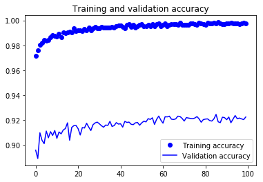
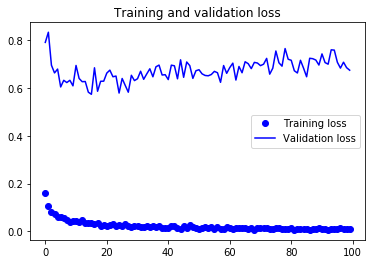
From the above two plots, you can see that the model is overfitting since there is a big gap between the training and validation loss. In order to address overfitting, you will have to maybe use some regularization techniques like Dropout. You can follow this tutorial on CNN in python with keras.

Model Evaluation on the Test Set

Finally, let's also evaluate your model on test data and see how it performs!

test_eval = full_model.evaluate(test_data, test_Y_one_hot, verbose=0)

print('Test loss:', test_eval[0])
print('Test accuracy:', test_eval[1])

('Test loss:', 0.7068972043234281)
('Test accuracy:', 0.9205)

Predict Labels

predicted_classes = full_model.predict(test_data)

Since the predictions you get are floating point values, it will not be feasible to compare the predicted labels with true test labels. So, you will round off the output which will convert the float values into an integer. Further, you will use np.argmax() to select the index number which has a higher value in a row.

For example, let's assume a prediction for one test image to be [0 1 0 0 0 0 0 0 0 0], the output for this should be a class label 1.

predicted_classes = np.argmax(np.round(predicted_classes),axis=1)

predicted_classes.shape, test_labels.shape

((10000,), (10000,))

correct = np.where(predicted_classes==test_labels)[0]
print "Found %d correct labels" % len(correct)
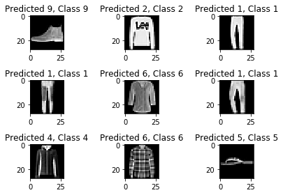
for i, correct in enumerate(correct[:9]):
    plt.subplot(3,3,i+1)
    plt.imshow(test_data[correct].reshape(28,28), cmap='gray', interpolation='none')
    plt.title("Predicted {}, Class {}".format(predicted_classes[correct], test_labels[correct]))
    plt.tight_layout()

Found 9204 correct labels

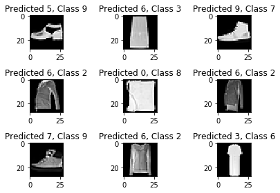
incorrect = np.where(predicted_classes!=test_labels)[0]
print "Found %d incorrect labels" % len(incorrect)
for i, incorrect in enumerate(incorrect[:9]):
    plt.subplot(3,3,i+1)
    plt.imshow(test_data[incorrect].reshape(28,28), cmap='gray', interpolation='none')
    plt.title("Predicted {}, Class {}".format(predicted_classes[incorrect], test_labels[incorrect]))
    plt.tight_layout()

Found 796 incorrect labels

Classification Report

Classification report will help you in identifying the misclassified classes in more detail. You will be able to observe for which class the model performed bad out of the given ten classes.

from sklearn.metrics import classification_report
target_names = ["Class {}".format(i) for i in range(num_classes)]
print(classification_report(test_labels, predicted_classes, target_names=target_names))

             precision    recall  f1-score   support

    Class 0       0.83      0.89      0.86      1000
    Class 1       0.99      0.99      0.99      1000
    Class 2       0.89      0.87      0.88      1000
    Class 3       0.92      0.93      0.92      1000
    Class 4       0.85      0.90      0.88      1000
    Class 5       0.99      0.99      0.99      1000
    Class 6       0.81      0.72      0.76      1000
    Class 7       0.96      0.98      0.97      1000
    Class 8       0.98      0.98      0.98      1000
    Class 9       0.98      0.96      0.97      1000

avg / total       0.92      0.92      0.92     10000

Would you like to dive deeper?

This tutorial was a good start of using both autoencoder and a fully connected convolutional neural network with Python and Keras. If you were able to follow along easily or even with little more efforts, well done! Try doing some experiments maybe with same model architecture but using different types of public datasets available.

There is still a lot to cover, so why not take DataCamp’s Deep Learning in Python course? In the meantime, also make sure to check out the Keras documentation, if you haven’t done so already. You will find more examples and information on all functions, arguments, more layers, etc. It will undoubtedly be an indispensable resource when you’re learning how to work with neural networks in Python!

If you rather feel like reading a book that explains the fundamentals of deep learning (with Keras) together with how it's used in practice, you should definitely read François Chollet's Deep Learning in Python book.