Course
You will use 3T brain MRI dataset to train your network. To observe the effectiveness of your model, you will be testing your model on:
- Unseen 3T MRI images,
- Noisy 3T MRI images and
- Use a qualitative metric: Peak signal to noise ratio (PSNR) to evaluate the performance of the reconstructed images.
This tutorial will not be addressing the intricacies of medical imaging but will be focused on the deep learning side! Note : This tutorial will mostly cover the practical implementation of convolutional autoencoders. So, if you are not yet aware about convolutional neural network (CNN) and autoencoder, you might want to look at CNN and Autoencoder tutorial. The best part about this tutorial is that you will be loading the 3D volumes as 2D images and will be feeding them in to the model. In a nutshull, you will address the following topics in today's tutorial:
- In the beginning you will be briefed about Magnetic Resonance Imaging (MRI),
- Then you will understand about the Brain MRI dataset: what kind of images it has, importing the modules, how to read the images, creating an array of the images, preprocessing the brain MRI images to be able to feed them in the model and finally explore the brain MRI images.
- In the implementation of convolutional autoencoder: you will fit the preprocessed data into the model, visualize the training and validation loss plot, sabe the trained model and finally predict on the test set.
- Next, you'll will test the robustness of your pre-trained model by adding noise into the test images and see how well the model performs quantitatively.
- Finally, you will test your predictions using a quantitative metric peak signal-to-noise ratio (PSNR) and measure the performance of your model.
Brief Introduction on MR images
A variety of systems are used in medical imaging ranging from open MRI units with magnetic field strength of 0.3 Tesla (T) to extremity MRI systems with field strengths up to 1.0 T and whole-body scanners with field strengths up to 3.0 T (in clinical use). Tesla is the unit of measuring the quantitative strength of magnetic field of MR images. High field MR scanners (7T, 11.5T) yielding higher SNR (signal-to-noise ratio) even with smaller voxel (a 3-dimensional patch or a grid) size and are thus preferred for more accurate diagnosis.
A smaller voxel size leads to a better resolution, which can in turn aid clinical diagnosis. However, the strength of magnetic field being used in MR scanner puts a lower bound on voxel size to maintain a good signal to noise ratio (SNR), in order to preserve the MR image details.
Despite the superior image quality of 7T and 11.5T, they are rarely deployed in production due to its cost constraints.
According to the recent papers, the reported number of 3T scanners are ~20,000 compared to just ~40 7T scanners.
Understanding the Brain MRI 3T Dataset
The brain MRI dataset consists of 3D volumes each volume has in total 207 slices/images of brain MRI's taken at different slices of the brain. Each slice is of dimension 173 x 173. The images are single channel grayscale images. There are in total 30 subjects, each subject containing the MRI scan of a patient. The image format is not jpeg,png etc. but rather nifti format. You will see in later section how to read the nifti format images.
The dataset consists of T1 modality MR images, T1 sequences are traditionally considered good for evaluation of anatomic structures. The dataset on which you will be working today consists of 3T Brain MRI's.
The dataset is public and is available for download at this source.
Tip: if you want to learn how to implement an Multi-Layer Perceptron (MLP) for classification tasks with the MNIST dataset, check out this tutorial.
Note : Before you begin please note that the model will be trained on a system with Nvidia 1080 Ti GPU Xeon e5 GeForce processor with 32GB RAM. If you are using Jupyter Notebook, you will need to add three more lines of code where you specify CUDA device order and CUDA visible devices using a module called os.
In the code below, you basically set environment variables in the notebook using os.environ. It's good to do the following before initializing Keras to limit Keras backend TensorFlow to use first GPU. If the machine on which you train on has a GPU on 0, make sure to use 0 instead of 1. You can check that by running a simple command on your terminal: for example, nvidia-smi
import os
os.environ["CUDA_DEVICE_ORDER"]="PCI_BUS_ID"
os.environ["CUDA_VISIBLE_DEVICES"]="1" #model will be trained on GPU 1
Importing the Modules
First, you import all the required modules like cv2, numpy, matplotlib and most importantly keras, since you'll be using that framework in today's tutorial!
In order to read the nifti format images, you also have to import a module called nibabel.
import os
import cv2
from keras.layers import Input,Dense,Flatten,Dropout,merge,Reshape,Conv2D,MaxPooling2D,UpSampling2D,Conv2DTranspose
from keras.layers.normalization import BatchNormalization
from keras.models import Model,Sequential
from keras.callbacks import ModelCheckpoint
from keras.optimizers import Adadelta, RMSprop,SGD,Adam
from keras import regularizers
from keras import backend as K
Using TensorFlow backend.
import numpy as np
import scipy.misc
import numpy.random as rng
from PIL import Image, ImageDraw, ImageFont
from sklearn.utils import shuffle
import nibabel as nib #reading MR images
from sklearn.cross_validation import train_test_split
import math
import glob
from matplotlib import pyplot as plt
%matplotlib inline
/usr/local/lib/python3.5/dist-packages/sklearn/cross_validation.py:44: DeprecationWarning: This module was deprecated in version 0.18 in favor of the model_selection module into which all the refactored classes and functions are moved. Also note that the interface of the new CV iterators are different from that of this module. This module will be removed in 0.20.
  "This module will be removed in 0.20.", DeprecationWarning)
Loading the Data
You will use glob module which will return a list comprising of all the volumes in the folder that you specify!
ff = glob.glob('ground3T/*')
Let's print the first element of the list and also check the length of the list: which in our case should be 30.
ff[0]
'ground3T/181232.nii.gz'
len(ff)
30
Now you are all set to load the 3D volumes using nibabel. Note that when you load a Nifti format volume, Nibabel does not load the image array. It waits until you ask for the array data. The normal way to ask for the array data is to call the get_data() method.
Since you want the 2D slices instead of 3D, you will initialise a list in which; every time you read a volume, you will iterate over all the complete 207 slices of the 3D volume and append each slice one by one in to a list.
images = []
Let's also print the shape of one of the 3D volume, it should be of the shape 173 x 207 x 173 (x, y, z; coordinates).
Note : You will be using only the middle 51 slices of the brain and not all the 207 slices. So, let's also see how to use only the center slices and load them.
for f in range(len(ff)):
    a = nib.load(ff[f])
    a = a.get_data()
    a = a[:,78:129,:]
    for i in range(a.shape[1]):
        images.append((a[:,i,:]))
print (a.shape)
(173, 51, 173)
Let's analyse shape of one slice out of 207 slices.
a[:,0,:].shape
(173, 173)
Data Preprocessing
Since images is a list you will use numpy module to convert the list in to a numpy array.
images = np.asarray(images)
It's time to check the shape of the numpy array, the first dimension of the array should be 207 x 30 = 6210 respectively and the remaining two dimensions will be 173 x 173.
images.shape
(1530, 173, 173)
The images of the dataset are indeed grayscale images with a dimension of 173 x 173 so before we feed the data into the model it is very important to preprocess it. You'll first convert each 173 x 173 image into a matrix of size 173 x 173 x 1, which you can feed into the network:
images = images.reshape(-1, 173,173,1)
images.shape
(1530, 173, 173, 1)
Next, rescale the data with using max-min normalisation technique:
m = np.max(images)
mi = np.min(images)
m, mi
(3599.0959, -341.83853)
images = (images - mi) / (m - mi)
Let's verify the minimum and maximum value of the data which should be 0.0 and 1.0 after rescaling it!
np.min(images), np.max(images)
(0.0, 1.0)
This is an important step, here you will pad the images with zeros at the boundaries so that the dimension of the images are even and it is easier to downsample the image by two while passing them through the model. Let's add zeros in three rows and three columns to make the dimension as 176 x 176
temp = np.zeros([1530,176,176,1])
temp[:,3:,3:,:] = images
images = temp
After all of this, it's important to partition the data. In order for your model to generalize well, you split the data into two parts: a training and a validation set. You will train your model on 80% of the data and validate it on 20% of the remaining training data.
This will also help you in reducing the chances of overfitting, as you will be validating your model on data it would not have seen in training phase.
You can use the train_test_split module of scikit-learn to divide the data properly:
from sklearn.model_selection import train_test_split
train_X,valid_X,train_ground,valid_ground = train_test_split(images,
                                                             images,
                                                             test_size=0.2,
                                                             random_state=13)
Note that for this task, you don't need training and testing labels. That's why you will pass the training images twice. Your training images will both act as the input as well as the ground truth similar to the labels you have in classification task.
Data Exploration
Let's now analyze how images in the dataset look like and also see the dimension of the images once again since you have added three extra rows and columns to the images with the help of the NumPy array attribute .shape:
# Shapes of training set
print("Dataset (images) shape: {shape}".format(shape=images.shape))
Dataset (images) shape: (1530, 176, 176, 1)
From the above output, you can see that the data has a shape of 6210 x 176 x 176 since there are 6210 samples each of 176 x 176 x 1 dimensional matrix.
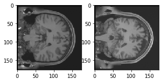
Now, let's take a look at couple of the training and validation images in your dataset:
plt.figure(figsize=[5,5])

# Display the first image in training data
plt.subplot(121)
curr_img = np.reshape(train_X[0], (176,176))
plt.imshow(curr_img, cmap='gray')

# Display the first image in testing data
plt.subplot(122)
curr_img = np.reshape(valid_X[0], (176,176))
plt.imshow(curr_img, cmap='gray')
<matplotlib.image.AxesImage at 0x7ff67d5d59b0>

The output of above two plots are from the training and validation set. You can see that both the training and validation images are different, it will be interesting to see if the convolutional autoencoder is able to learn the features and is reconstructing these images properly.
Now you are all set to define the network and feed the data into the network. So without any further ado, let's jump to the next step!
The Convolutional Autoencoder!
The images are of size 176 x 176 x 1 or a 30976-dimensional vector. You convert the image matrix to an array, rescale it between 0 and 1, reshape it so that it's of size 176 x 176 x 1, and feed this as an input to the network.
Also, you will use a batch size of 128 using a higher batch size of 256 or 512 is also preferable it all depends on the system you train your model. It contributes heavily in determining the learning parameters and affects the prediction accuracy. You will train your network for 50 epochs.
batch_size = 128
epochs = 300
inChannel = 1
x, y = 176, 176
input_img = Input(shape = (x, y, inChannel))
As you might already know well before, the autoencoder is divided into two parts: there's an encoder and a decoder.
Encoder: It has 3 Convolution blocks, each block has a convolution layer followed a batch normalization layer. Max-pooling layer is used after the first and second convolution blocks.
- The first convolution block will have 32 filters of size 3 x 3, followed by a downsampling (max-pooling) layer,
- The second block will have 64 filters of size 3 x 3, followed by another downsampling layer,
- The final block of encoder will have 128 filters of size 3 x 3.
Decoder: It has 2 Convolution blocks, each block has a convolution layer followed a batch normalization layer. Upsampling layer is used after the first and second convolution blocks.
- The first block will have 128 filters of size 3 x 3 followed by a upsampling layer,
- The second block will have 64 filters of size 3 x 3 followed by another upsampling layer,
- The final layer of encoder will have 1 filter of size 3 x 3 which will reconstruct back the input having a single channel.
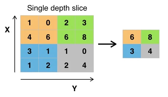
The max-pooling layer will downsample the input by two times each time you use it, while the upsampling layer will upsample the input by two times each time it is used.
Note: The number of filters, the filter size, the number of layers, number of epochs you train your model, are all hyperparameters and should be decided based on your own intuition, you are free to try new experiments by tweaking with these hyperparameters and measure the performance of your model. And that is how you will slowly learn the art of deep learning!
def autoencoder(input_img):
    #encoder
    #input = 28 x 28 x 1 (wide and thin)
    conv1 = Conv2D(32, (3, 3), activation='relu', padding='same')(input_img) #28 x 28 x 32
    conv1 = BatchNormalization()(conv1)
    conv1 = Conv2D(32, (3, 3), activation='relu', padding='same')(conv1)
    conv1 = BatchNormalization()(conv1)
    pool1 = MaxPooling2D(pool_size=(2, 2))(conv1) #14 x 14 x 32
    conv2 = Conv2D(64, (3, 3), activation='relu', padding='same')(pool1) #14 x 14 x 64
    conv2 = BatchNormalization()(conv2)
    conv2 = Conv2D(64, (3, 3), activation='relu', padding='same')(conv2)
    conv2 = BatchNormalization()(conv2)
    pool2 = MaxPooling2D(pool_size=(2, 2))(conv2) #7 x 7 x 64
    conv3 = Conv2D(128, (3, 3), activation='relu', padding='same')(pool2) #7 x 7 x 128 (small and thick)
    conv3 = BatchNormalization()(conv3)
    conv3 = Conv2D(128, (3, 3), activation='relu', padding='same')(conv3)
    conv3 = BatchNormalization()(conv3)


    #decoder
    conv4 = Conv2D(64, (3, 3), activation='relu', padding='same')(conv3) #7 x 7 x 128
    conv4 = BatchNormalization()(conv4)
    conv4 = Conv2D(64, (3, 3), activation='relu', padding='same')(conv4)
    conv4 = BatchNormalization()(conv4)
    up1 = UpSampling2D((2,2))(conv4) # 14 x 14 x 128
    conv5 = Conv2D(32, (3, 3), activation='relu', padding='same')(up1) # 14 x 14 x 64
    conv5 = BatchNormalization()(conv5)
    conv5 = Conv2D(32, (3, 3), activation='relu', padding='same')(conv5)
    conv5 = BatchNormalization()(conv5)
    up2 = UpSampling2D((2,2))(conv5) # 28 x 28 x 64
    decoded = Conv2D(1, (3, 3), activation='sigmoid', padding='same')(up2) # 28 x 28 x 1
    return decoded
After the model is created, you have to compile it using the optimizer to be RMSProp.
Note that you also have to specify the loss type via the argument loss. In this case, that's the mean squared error, since the loss after every batch will be computed between the batch of predicted output and the ground truth using mean squared error pixel by pixel:
autoencoder = Model(input_img, autoencoder(input_img))
autoencoder.compile(loss='mean_squared_error', optimizer = RMSprop())
Let's visualize the layers that you created in the above step by using the summary function, this will show number of parameters (weights and biases) in each layer and also the total parameters in your model.
autoencoder.summary()
_________________________________________________________________
Layer (type)                 Output Shape              Param #
=================================================================
input_2 (InputLayer)         (None, 176, 176, 1)       0
_________________________________________________________________
conv2d_18 (Conv2D)           (None, 176, 176, 32)      320
_________________________________________________________________
batch_normalization_11 (Batc (None, 176, 176, 32)      128
_________________________________________________________________
conv2d_19 (Conv2D)           (None, 176, 176, 32)      9248
_________________________________________________________________
batch_normalization_12 (Batc (None, 176, 176, 32)      128
_________________________________________________________________
max_pooling2d_5 (MaxPooling2 (None, 88, 88, 32)        0
_________________________________________________________________
conv2d_20 (Conv2D)           (None, 88, 88, 64)        18496
_________________________________________________________________
batch_normalization_13 (Batc (None, 88, 88, 64)        256
_________________________________________________________________
conv2d_21 (Conv2D)           (None, 88, 88, 64)        36928
_________________________________________________________________
batch_normalization_14 (Batc (None, 88, 88, 64)        256
_________________________________________________________________
max_pooling2d_6 (MaxPooling2 (None, 44, 44, 64)        0
_________________________________________________________________
conv2d_22 (Conv2D)           (None, 44, 44, 128)       73856
_________________________________________________________________
batch_normalization_15 (Batc (None, 44, 44, 128)       512
_________________________________________________________________
conv2d_23 (Conv2D)           (None, 44, 44, 128)       147584
_________________________________________________________________
batch_normalization_16 (Batc (None, 44, 44, 128)       512
_________________________________________________________________
conv2d_24 (Conv2D)           (None, 44, 44, 64)        73792
_________________________________________________________________
batch_normalization_17 (Batc (None, 44, 44, 64)        256
_________________________________________________________________
conv2d_25 (Conv2D)           (None, 44, 44, 64)        36928
_________________________________________________________________
batch_normalization_18 (Batc (None, 44, 44, 64)        256
_________________________________________________________________
up_sampling2d_5 (UpSampling2 (None, 88, 88, 64)        0
_________________________________________________________________
conv2d_26 (Conv2D)           (None, 88, 88, 32)        18464
_________________________________________________________________
batch_normalization_19 (Batc (None, 88, 88, 32)        128
_________________________________________________________________
conv2d_27 (Conv2D)           (None, 88, 88, 32)        9248
_________________________________________________________________
batch_normalization_20 (Batc (None, 88, 88, 32)        128
_________________________________________________________________
up_sampling2d_6 (UpSampling2 (None, 176, 176, 32)      0
_________________________________________________________________
conv2d_28 (Conv2D)           (None, 176, 176, 1)       289
=================================================================
Total params: 427,713
Trainable params: 426,433
Non-trainable params: 1,280
_________________________________________________________________
It's finally time to train the model with Keras' fit() function! The model trains for 50 epochs. The fit() function will return a history object; By storying the result of this function in fashion_train, you can use it later to plot the loss function plot between training and validation which will help you to analyze your model's performance visually.
Train the Model
autoencoder_train = autoencoder.fit(train_X, train_ground, batch_size=batch_size,epochs=epochs,verbose=1,validation_data=(valid_X, valid_ground))
Train on 1224 samples, validate on 306 samples
Epoch 1/300
1224/1224 [==============================] - 7s - loss: 0.1201 - val_loss: 0.0838
Epoch 2/300
1224/1224 [==============================] - 7s - loss: 0.0492 - val_loss: 0.0534
...
Epoch 299/300
1224/1224 [==============================] - 7s - loss: 1.3101e-04 - val_loss: 6.1086e-04
Epoch 300/300
1224/1224 [==============================] - 7s - loss: 1.0711e-04 - val_loss: 3.9641e-04
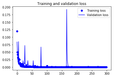
Finally! You trained the model on the fingerprint dataset for 200 epochs, Now, let's plot the loss plot between training and validation data to visualise the model performance.
loss = autoencoder_train.history['loss']
val_loss = autoencoder_train.history['val_loss']
epochs = range(300)
plt.figure()
plt.plot(epochs, loss, 'bo', label='Training loss')
plt.plot(epochs, val_loss, 'b', label='Validation loss')
plt.title('Training and validation loss')
plt.legend()
plt.show()

Finally, you can see that the validation loss and the training loss both are in sync. It shows that your model is not overfitting: the validation loss is decreasing and not increasing, and there is rarely any gap between training and validation loss throughout the training phase.
Therefore, you can say that your model's generalization capability is good.
Finally, it's time to reconstruct the test images using the predict() function of Keras and see how well your model is able reconstruct on the test data.
Save the Model
Let's now save the trained model. It is an important step when you are working with Deep Learning.Since, the weights are the heart of the solution to the problem you are tackling at hand!
You can anytime load the saved weights in the same model and train it from where your training stopped. For example: The above model if trained again, the parameters like weights, biases, the loss function etc. will not start from the beginning and it will no more be a fresh training.
Within just one line of code you can save and load back the weights into the model.
autoencoder = autoencoder.save_weights('autoencoder_mri.h5')
autoencoder = Model(input_img, autoencoder(input_img))
autoencoder.load_weights('autoencoder_mri.h5')
Predicting on Validation Data
Since here you do not have a testing data. Let's use the validation data for predicting on the model that you trained just now.
You will be predicting the trained model on the remaining 306 validation images and plot few of the reconstructed images to visualize how well your model is able to reconstruct the validation images.
pred = autoencoder.predict(valid_X)
plt.figure(figsize=(20, 4))
print("Test Images")
for i in range(5):
    plt.subplot(1, 5, i+1)
    plt.imshow(valid_ground[i, ..., 0], cmap='gray')
plt.show()
plt.figure(figsize=(20, 4))
print("Reconstruction of Test Images")
for i in range(5):
    plt.subplot(1, 5, i+1)
    plt.imshow(pred[i, ..., 0], cmap='gray')
plt.show()
Test Images

Reconstruction of Test Images

From the above figures, you can observe that your model did a fantastic job in reconstructing the test images that you predicted using the model. At least qualitatively, the test and the reconstructed images look almost exactly similar.
May be it can do a bit better job on reconstructing some local details present in the original 3T images.
Predicting on Noisy 3T images
First let's add some noise into the validation images with a mean zero and standard deviation of 0.03.
[a,b,c,d]= np.shape(valid_X)
mean = 0
sigma = 0.03
gauss = np.random.normal(mean,sigma,(a,b,c,d))
noisy_images = valid_X + gauss
Its time to do prediction on the noisy validation images. Let's see how well your model does on noisy images despite of not being trained on them.
pred_noisy = autoencoder.predict(noisy_images)
plt.figure(figsize=(20, 4))
print("Noisy Test Images")
for i in range(5):
    plt.subplot(1, 5, i+1)
    plt.imshow(noisy_images[i, ..., 0], cmap='gray')
plt.show()
plt.figure(figsize=(20, 4))
print("Reconstruction of Noisy Test Images")
for i in range(5):
    plt.subplot(1, 5, i+1)
    plt.imshow(pred_noisy[i, ..., 0], cmap='gray')
plt.show()
Noisy Test Images

Reconstruction of Noisy Test Images

It seems the model did a pretty good job. Isn't it? After all the reconstructed images look better than the noisy images. Moreover, the model never actually saw the noisy images while being trained.
Quantitative Metric: Peak Signal-to-Noise Ratio (PSNR)
The PSNR block computes the peak signal-to-noise ratio, in decibels(dB), between two images. This ratio is often used as a quality measurement between the original and a reconstructed image. The higher the PSNR, the better the quality of the reconstructed image.
So, first let's compute the performance of the validation and the reconstructed validation images.
valid_pred = autoencoder.predict(valid_X)
mse =  np.mean((valid_X - valid_pred) ** 2)
psnr = 20 * math.log10( 1.0 / math.sqrt(mse))
print('PSNR of reconstructed validation images: {psnr}dB'.format(psnr=np.round(psnr,2)))
PSNR of reconstructed validation images: 34.02dB
Next, let us compute the PSNR between the original validation and the predicted noisy images
noisy_pred = autoencoder.predict(noisy_images)
mse =  np.mean((valid_X - noisy_pred) ** 2)
psnr_noisy = 20 * math.log10( 1.0 / math.sqrt(mse))
print('PSNR of reconstructed validation images: {psnr}dB'.format(psnr=np.round(psnr_noisy,2)))
PSNR of reconstructed validation images: 32.48dB
Well, looks like quantitatively there is merely a difference of 1.54 dB between the PSNR of without noise reconstructions and with noise reconstructions. Moreover, you have not trained your model to handle noise. Isn't this amazing?
Go Further!
This tutorial was good start to understanding how to read MRI nifti format images, analyse, preprocess and feed them into the model using a brain MRI 3T dataset. It showed you one of the nice application of autoencoders practically. If you were able to follow along easily or even with little more efforts, well done!
You can play around with the architecture and try improving the predictions both quantitatively and qualitatively. May be by adding more layers, may be by training it for more time? Try these combinations and see if that helps.
There is still a lot to cover, so why not take DataCamp’s Deep Learning in Python course? If you haven’t done so already. You will learn from the basics and slowly will move into mastering the deep learning domain, it will undoubtedly be an indispensable resource when you’re learning how to work with convolutional neural networks in Python, how to detect faces, objects etc.

