Course
Introduction to Python
4 hr
6.9M
You will use FVC2002 fingerprint dataset to train your network. To observe the effectiveness of your model, you will be testing your model on two different fingerprint sensor datasets namely Secugen and Lumidigm sensor.
Note : This tutorial will mostly cover the practical implementation of convolutional autoencoders. So, if you are not yet aware of convolutional neural network (CNN) and autoencoder, you might want to look at CNN and Autoencoder tutorial.
To encapsulate, you will address the following topics in today's tutorial:
Before you go ahead and load in the data, it's good to take a look at what you'll exactly be working with! The FVC2002 fingerprint dataset is a Fingerprint Verification Competition dataset which was organized back in the year 2000 and then again in the year 2002. This dataset consists of four different sensor fingerprints namely Low-cost Optical Sensor, Low-cost Capacitive Sensor, Optical Sensor and Synthetic Generator, each sensor having varying image sizes. The dataset has 3200 images in set A, 800 images per sensor. You can double check this later when you have loaded in your data! ;)
The Fingerprint dataset is not predefined in the Keras or the TensorFlow framework, so you'll have to download the data from this source. You'll see how this works in the next section!
Note : Before you begin, please note that the model will be trained on a system with Nvidia 1080 Ti GPU Xeon e5 GeForce processor with 32GB RAM. If you are using Jupyter Notebook, you will need to add three more lines of code where you specify CUDA device order and CUDA visible devices using a module called os.
In the code below, you basically set environment variables in the notebook using os.environ. It's good to do the following before initializing Keras to limit Keras backend TensorFlow to use the first GPU. If the machine on which you train on has a GPU on 0, make sure to use 0 instead of 1. You can check that by running a simple command on your terminal: for example, nvidia-smi
import os
os.environ["CUDA_DEVICE_ORDER"]="PCI_BUS_ID"
os.environ["CUDA_VISIBLE_DEVICES"]="1" #model will be trained on GPU 1
First, you import all the required modules like cv2, numpy, matplotlib and most importantly keras, since you'll be using that framework in today's tutorial!
import cv2
import matplotlib.pyplot as plt
%matplotlib inline
from skimage.filters import threshold_otsu
import numpy as np
from glob import glob
from scipy import misc
from matplotlib.patches import Circle,Ellipse
from matplotlib.patches import Rectangle
import os
from PIL import Image
import keras
from matplotlib import pyplot as plt
import numpy as np
import gzip
%matplotlib inline
from keras.layers import Input,Conv2D,MaxPooling2D,UpSampling2D
from keras.models import Model
from keras.optimizers import RMSprop
from keras.layers.normalization import BatchNormalization
Using TensorFlow backend.
data = glob('FVC2002/Db*/*')
len(data)
3200
images = []
def read_images(data):
    for i in range(len(data)):
        img = misc.imread(data[i])
        img = misc.imresize(img,(224,224))
        images.append(img)
    return images
images = read_images(data)
images_arr = np.asarray(images)
images_arr = images_arr.astype('float32')
images_arr.shape
(3200, 224, 224)
Once you have the data loaded, you are all set to analyze the data in order to get some intuition about the dataset that you are going to work with for today's tutorial!
Let's now analyze how images in the dataset look like and also see the dimension of the images with the help of the NumPy array attribute .shape:
# Shapes of training set
print("Dataset (images) shape: {shape}".format(shape=images_arr.shape))
Dataset (images) shape: (3200, 224, 224)
From the above output, you can see that the data has a shape of 3200 x 224 x 224 since there are 3200 samples each of 224 x 224 dimensional matrix.
Now, let's take a look at a couple of the images in your dataset:
#plt.figure(figsize=[5,5])

# Display the first image in training data
for i in range(2):
    plt.figure(figsize=[5, 5])
    curr_img = np.reshape(images_arr[i], (224,224))
    plt.imshow(curr_img, cmap='gray')
    plt.show()
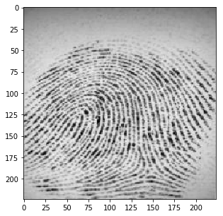
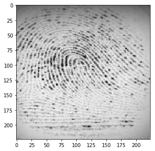
The output of the above two plots are from the dataset. You can see that the fingerprints are not very clear, it will be interesting to see if the convolutional autoencoder is able to learn the features and is reconstructing these images properly.
The images of the dataset are indeed grayscale images with pixel values ranging from 0 to 255 with a dimension of 224 x 224, so before you feed the data into the model, it is very important to preprocess it. You'll first convert each 224 x 224 image of the dataset into a matrix of size 224 x 224 x 1, which you can then feed into the network:
images_arr = images_arr.reshape(-1, 224,224, 1)
images_arr.shape
(3200, 224, 224, 1)
Next, you want to make sure to check the data type of the NumPy array; it should be in float32 format, if not you will need to convert it into this format, you also have to rescale the pixel values in range 0 - 1 inclusive. So let's do that!
First, let's verify the data type:
images_arr.dtype
dtype('float32')
Next, rescale the data with the maximum pixel value of the images in the data:
np.max(images_arr)
255.0
images_arr = images_arr / np.max(images_arr)
Let's verify the maximum and minimum value of data which should be 0.0 and 1.0 after rescaling it!
np.max(images_arr), np.min(images_arr)
(1.0, 0.0)
After all of this, it's important to partition the data. In order for your model to generalize well, you split the data into two parts: training and a validation set. You will train your model on 80% of the data and validate it on 20% of the remaining training data.
This will also help you in reducing the chances of overfitting, as you will be validating your model on data it would not have seen in the training phase.
You can use the train_test_split module of scikit-learn to divide the data properly:
from sklearn.model_selection import train_test_split
train_X,valid_X,train_ground,valid_ground = train_test_split(images_arr,
                                                             images_arr,
                                                             test_size=0.2,
                                                             random_state=13)
Note that for this task, you don't need training and testing labels. That's why you will pass the training images twice. Your training images will both act as the input as well as the ground truth similar to the labels you have in the classification task.
Now you are all set to define the network and feed the data into the network. So without any further ado, let's jump to the next step!
The images are of size 224 x 224 x 1 or a 50,176-dimensional vector. You convert the image matrix to an array, rescale it between 0 and 1, reshape it so that it's of size 224 x 224 x 1, and feed this as an input to the network.
Also, you will use a batch size of 128 using a higher batch size of 256 or 512 is also preferable it all depends on the system you train your model. It contributes heavily in determining the learning parameters and affects the prediction accuracy. You will train your network for 50 epochs.
batch_size = 128
epochs = 200
inChannel = 1
x, y = 224, 224
input_img = Input(shape = (x, y, inChannel))
As you might already know well before, the autoencoder is divided into two parts: there is an encoder and a decoder.
Encoder
Decoder
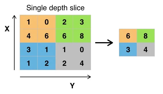
The max-pooling layer will downsample the input by two times each time you use it, while the upsampling layer will upsample the input by two times each time it is used.
Note: The number of filters, the filter size, the number of layers, number of epochs you train your model, are all hyperparameters and should be decided based on your own intuition, you are free to try new experiments by tweaking with these hyperparameters and measure the performance of your model. And that is how you will slowly learn the art of deep learning!
def autoencoder(input_img):
    #encoder
    #input = 28 x 28 x 1 (wide and thin)
    conv1 = Conv2D(32, (3, 3), activation='relu', padding='same')(input_img) #28 x 28 x 32
    pool1 = MaxPooling2D(pool_size=(2, 2))(conv1) #14 x 14 x 32
    conv2 = Conv2D(64, (3, 3), activation='relu', padding='same')(pool1) #14 x 14 x 64
    pool2 = MaxPooling2D(pool_size=(2, 2))(conv2) #7 x 7 x 64
    conv3 = Conv2D(128, (3, 3), activation='relu', padding='same')(pool2) #7 x 7 x 128 (small and thick)

    #decoder
    conv4 = Conv2D(128, (3, 3), activation='relu', padding='same')(conv3) #7 x 7 x 128
    up1 = UpSampling2D((2,2))(conv4) # 14 x 14 x 128
    conv5 = Conv2D(64, (3, 3), activation='relu', padding='same')(up1) # 14 x 14 x 64
    up2 = UpSampling2D((2,2))(conv5) # 28 x 28 x 64
    decoded = Conv2D(1, (3, 3), activation='sigmoid', padding='same')(up2) # 28 x 28 x 1
    return decoded
After the model is created, you have to compile it using the optimizer to be RMSProp.
Note that you also have to specify the loss type via the argument loss. In this case, that's the mean squared error, since the loss after every batch will be computed between the batch of predicted output and the ground truth using mean squared error pixel by pixel:
autoencoder = Model(input_img, autoencoder(input_img))
autoencoder.compile(loss='mean_squared_error', optimizer = RMSprop())
Let's visualize the layers that you created in the above step by using the summary function; this will show a number of parameters (weights and biases) in each layer and also the total parameters in your model.
autoencoder.summary()
_________________________________________________________________
Layer (type)                 Output Shape              Param #
=================================================================
input_1 (InputLayer)         (None, 224, 224, 1)       0
_________________________________________________________________
conv2d_1 (Conv2D)            (None, 224, 224, 32)      320
_________________________________________________________________
max_pooling2d_1 (MaxPooling2 (None, 112, 112, 32)      0
_________________________________________________________________
conv2d_2 (Conv2D)            (None, 112, 112, 64)      18496
_________________________________________________________________
max_pooling2d_2 (MaxPooling2 (None, 56, 56, 64)        0
_________________________________________________________________
conv2d_3 (Conv2D)            (None, 56, 56, 128)       73856
_________________________________________________________________
conv2d_4 (Conv2D)            (None, 56, 56, 128)       147584
_________________________________________________________________
up_sampling2d_1 (UpSampling2 (None, 112, 112, 128)     0
_________________________________________________________________
conv2d_5 (Conv2D)            (None, 112, 112, 64)      73792
_________________________________________________________________
up_sampling2d_2 (UpSampling2 (None, 224, 224, 64)      0
_________________________________________________________________
conv2d_6 (Conv2D)            (None, 224, 224, 1)       577
=================================================================
Total params: 314,625
Trainable params: 314,625
Non-trainable params: 0
_________________________________________________________________
It's finally time to train the model with Keras' fit() function! The model trains for 200 epochs. The fit() function will return a history object; By storing the result of this function in fashion_train, you can use it later to plot the loss function plot between training and validation which will help you to analyze your model's performance visually.
autoencoder_train = autoencoder.fit(train_X, train_ground, batch_size=batch_size,epochs=epochs,verbose=1,validation_data=(valid_X, valid_ground))
Train on 2560 samples, validate on 640 samples
Epoch 1/200
2560/2560 [==============================] - 17s - loss: 0.0677 - val_loss: 0.0498
Epoch 2/200
2560/2560 [==============================] - 11s - loss: 0.0369 - val_loss: 0.0287
...
2560/2560 [==============================] - 11s - loss: 0.0029 - val_loss: 0.0024
Epoch 200/200
2560/2560 [==============================] - 11s - loss: 0.0027 - val_loss: 0.0028
Finally! You trained the model on the fingerprint dataset for 200 epochs, Now, let's plot the loss plot between training and validation data to visualize the model performance.
loss = autoencoder_train.history['loss']
val_loss = autoencoder_train.history['val_loss']
epochs = range(200)
plt.figure()
plt.plot(epochs, loss, 'bo', label='Training loss')
plt.plot(epochs, val_loss, 'b', label='Validation loss')
plt.title('Training and validation loss')
plt.legend()
plt.show()
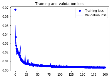
Finally, you can see that the validation loss and the training loss both are in sync. It shows that your model is not overfitting: the validation loss is decreasing and not increasing, and there is rarely any gap between training and validation loss especially as the training proceeds after 40th epoch.
Therefore, you can say that your model's generalization capability is good.
Finally, it's time to reconstruct the test images using the predict() function of Keras and see how well your model is able to reconstruct on the test data.
Let's now save the trained model. It is an important step when you are working with Deep Learning. Since the weights are the heart of the solution to the problem you are tackling at hand!
You can anytime load the saved weights in the same model and train it from where your training stopped. For example, the above model if trained again, the parameters like weights, biases, the loss function, etc. will not start from the beginning and it will no longer be a fresh training.
Within just one line of code, you can save and load back the weights into the model.
autoencoder = autoencoder.save_weights('autoencoder.h5')
autoencoder = Model(input_img, autoencoder(input_img))
autoencoder.load_weights('autoencoder.h5')
autoencoder.compile(loss='mean_squared_error', optimizer = RMSprop())
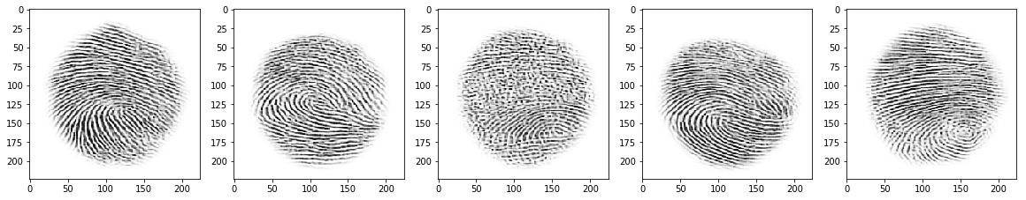
Since here you do not have a testing data. Let's use the validation data for predicting on the model that you trained just now.
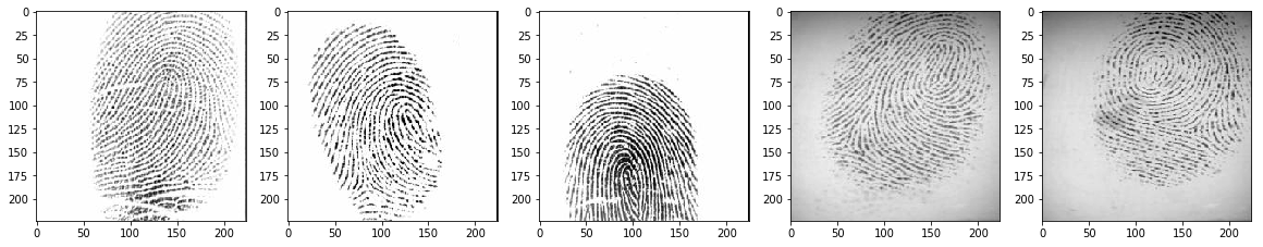
You will be predicting the trained model on the remaining 640 validation images and plot few of the reconstructed images to visualize how well your model is able to reconstruct the validation images.
pred = autoencoder.predict(valid_X)
plt.figure(figsize=(20, 4))
print("Test Images")
for i in range(5):
    plt.subplot(1, 5, i+1)
    plt.imshow(valid_ground[i, ..., 0], cmap='gray')
plt.show()
plt.figure(figsize=(20, 4))
print("Reconstruction of Test Images")
for i in range(5):
    plt.subplot(1, 5, i+1)
    plt.imshow(pred[i, ..., 0], cmap='gray')
plt.show()
Test Images
Reconstruction of Test Images
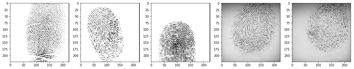
From the above figures, you can observe that your model did a fantastic job of reconstructing the test images that you predicted using the model. At least visually, the test and the reconstructed images look almost exactly similar.
As you saw in the training vs. validation plot that your model was generalizing well on the unseen data. It is now time to test its robustness with altogether a different sensor data.
You will be testing your model on two different types of sensors.
First, let's test your model on a low-quality fingerprint sensor data i.e. Secugen and see how well the model performs!
sec = glob('Secugen/*')
images = []
def read_images(data):
    for i in range(len(data)):
        img = misc.imread(data[i])
        img = misc.imresize(img,(224,224))
        images.append(img)
    return images
images = read_images(sec)
secugen = np.asarray(images)
secugen = secugen.astype('float32')
images_arr.shape
(48, 224, 224, 1)
secugen = secugen / np.max(secugen)
secugen = secugen.reshape(-1, 224,224, 1)
pred = autoencoder.predict(secugen)
plt.figure(figsize=(20, 4))
print("Test Secugen Images")
for i in range(5):
    plt.subplot(1, 5, i+1)
    plt.imshow(secugen[i, ..., 0], cmap='gray')
plt.show()
plt.figure(figsize=(20, 4))
print("Reconstruction of Test Secugen Images")
for i in range(5):
    plt.subplot(1, 5, i+1)
    plt.imshow(pred[i, ..., 0], cmap='gray')
plt.show()
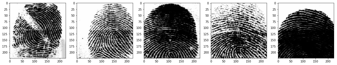
Test Secugen Images
Reconstruction of Test Secugen Images
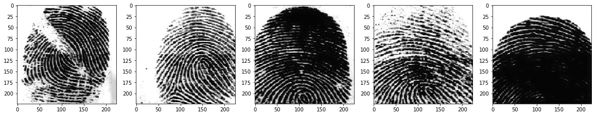
From the above figures, you can observe that your model did a great job in reconstructing the secugen images that you predicted using the trained model. Isn't that amazing?
Now, let's test your model on a fairly better quality sensor images i.e.Lumidigm
lum = glob('Lumidigm/*')
images = []
def read_images(data):
    for i in range(len(data)):
        img = misc.imread(data[i])
        img = misc.imresize(img,(224,224))
        images.append(img)
    return images
images = read_images(lum)
lumidigm = np.asarray(images)
lumidigm = lumidigm.astype('float32')
lumidigm.shape
(48, 224, 224)
lumidigm = lumidigm / np.max(lumidigm)
lumidigm = lumidigm.reshape(-1, 224,224, 1)
pred = autoencoder.predict(lumidigm)
plt.figure(figsize=(20, 4))
print("Test Lumidigm Images")
for i in range(5):
    plt.subplot(1, 5, i+1)
    plt.imshow(lumidigm[i, ..., 0], cmap='gray')
plt.show()
plt.figure(figsize=(20, 4))
print("Reconstruction of Test Lumidigm Images")
for i in range(5):
    plt.subplot(1, 5, i+1)
    plt.imshow(pred[i, ..., 0], cmap='gray')
plt.show()
Test Lumidigm Images

Reconstruction of Test Lumidigm Images
From the above figures, you can observe that your model again did an excellent job in reconstructing the lumidigm images as well that you predicted using the trained model.
This tutorial was a good start to understanding how to read images from scratch, analyze, preprocess and feed them into the model using a fingerprint dataset. It showed you one of the nice application of autoencoders practically. If you were able to follow along easily or even with a little more effort, well done!
In the next tutorial, you will be learning how to read medical images of T-1 modality and reconstruct them using an autoencoder!
There is still a lot to cover, so why not take DataCamp’s Deep Learning in Python course? If you haven’t done so already. You will learn from the basics and slowly will move into mastering the deep learning domain; it will undoubtedly be an indispensable resource when you’re learning how to work with convolutional neural networks in Python, how to detect faces, objects, etc.
Python Courses
Course
Course
Course
Tutorial
Aditya Sharma
Tutorial
Aditya Sharma
Tutorial
Aditya Sharma
Tutorial
Aditya Sharma
Tutorial
Aditya Sharma
Tutorial
Natassha Selvaraj