MongoDB Aggregation Pipeline Tutorial in Python with PyMongo

Working with large datasets often presents the challenge of extracting meaningful patterns and insights while maintaining performance. When your applications store data in MongoDB, running complex queries and transformations directly in the database can be much faster than moving data to external analysis tools. MongoDB aggregation pipelines provide a solution by letting you process, transform, and analyze data right where it lives.

You can create custom data processing workflows by connecting simple operations in sequence. Each stage in the pipeline transforms documents and passes results to the next stage. For instance, you might need to filter records by date range, group them by category, calculate statistical measures, and format the output — all accomplished through a single database operation that processes data close to its source.

In this article, you’ll learn how to build aggregation pipelines to solve common data challenges, with all examples demonstrated in PyMongo (MongoDB’s official Python client). 

While this article focuses on aggregation pipelines, if you’re new to using MongoDB with Python, the Introduction to MongoDB in Python course offers a comprehensive starting point. You’ll gain enough foundation from this article to translate these aggregation concepts to MongoDB’s query language on your own or with help from language models.

What are Aggregation Pipelines in MongoDB?

Picture yourself needing to analyze customer reviews across multiple products to understand satisfaction trends. Traditional queries might retrieve the data, but they don’t help with combining, analyzing, and transforming that information into useful summaries. 

MongoDB’s aggregation pipelines solve this by providing a structured way to process data through a series of operations that build on each other.

Pipeline architecture and document flow

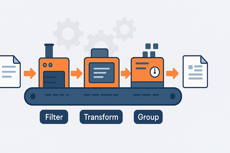
Think of aggregation pipelines as assembly lines for your data. Each document from your collection enters one end of the pipeline and passes through various stations (stages) where it gets filtered, transformed, grouped, or enriched. 

The output from one stage becomes the input for the next, allowing you to break complex data transformations into smaller, manageable steps.

These pipelines use a declarative approach ;  you specify what you want at each stage rather than how to compute it. This approach makes your data processing intentions clear and allows MongoDB to handle the execution details. The database can then apply various optimizations based on your pipeline structure.

Stage order matters in your pipeline design. Filtering documents early (before grouping or complex calculations) reduces the amount of data flowing through the pipeline. 

This approach can dramatically improve performance when working with large collections. A well-structured pipeline processes only the data needed for your final results.

• Document flow: Documents enter → transform through stages → results emerge
• Declarative design: Specify what you want, not how to compute it
• Ordered processing: Each stage’s output feeds directly into the next stage
• Performance benefit: Early filtering reduces data volume in later stages

Stage typology and functional categories

MongoDB aggregation stages fall into four main categories based on their purpose. Filtering stages like $match work like queries, selecting only documents that meet specific criteria. This helps narrow down your dataset before performing more complex operations.

Reshaping stages transform document structure. Using $project or $addFields, you can include, exclude, or rename fields, or create calculated fields based on existing values. These stages help simplify documents by keeping only relevant information and adding computed values needed for analysis.

When you need to combine multiple documents based on shared characteristics, grouping stages come into play. The $group stage is the workhorse here, allowing you to calculate counts, sums, averages, and other aggregated values across groups of documents. This transforms thousands of individual records into meaningful summaries that answer your analytical questions.

To complete your data picture, join stages like $lookup allows you to combine information from multiple collections. This lets you enrich documents with related data, similar to SQL joins but adapted for MongoDB's document model. The ability to reference data across collections helps maintain proper data normalization while still delivering complete results in a single operation.

• Filtering: Select specific documents with $match based on criteria
• Reshaping: Transform document structure with $project and $addFields
• Grouping: Combine and summarize with $group for aggregated values
• Joining: Connect related data across collections with $lookup

For a complete reference on capabilities and operators, you can consult the MongoDB Aggregation Pipeline Manual.

Setting Up the Environment For the Tutorial

Before diving into MongoDB aggregation pipelines, you need a working environment with PyMongo and access to a sample dataset. This section walks you through the setup process with the sample_analytics dataset, which contains financial data perfect for demonstrating aggregation concepts.

Installing PyMongo

PyMongo is MongoDB’s official Python driver. You can install it using pip on both macOS and Windows:

# Install PyMongo using pip
pip install pymongo

# Or if you're using conda
conda install -c conda-forge pymongo

• Version compatibility: PyMongo 4.x works with Python 3.7+
• Dependency handling: The installer automatically handles required dependencies
• Platform support: Works identically across Windows, macOS, and Linux

Accessing the sample dataset

MongoDB offers sample datasets that you can use without creating your own data. The easiest approach is using MongoDB Atlas (the cloud version):

1. Create a free MongoDB Atlas account at mongodb.com/cloud/atlas
2. Set up a free tier cluster

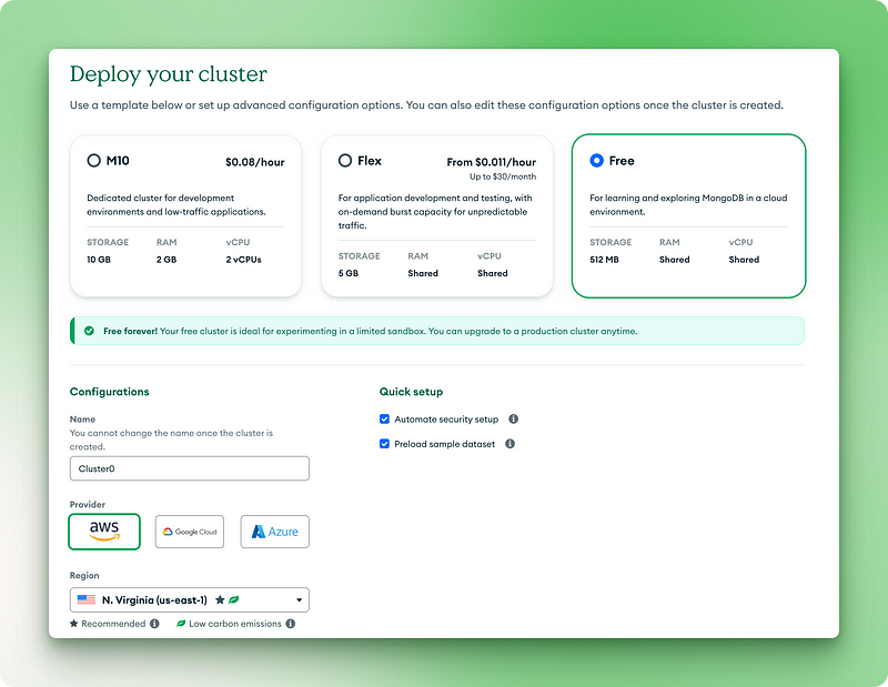
2.1. Choose the free forever version

2.2. Name your cluster

2.3. Click “Deploy”

2.4. Copy your username and password to somewhere secure

2.5. Click “Create database user”

2.6. Choose “Drivers” for your connection method

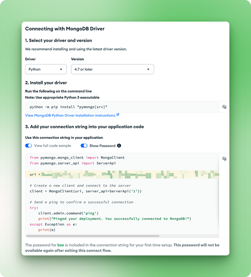
2.7. Copy the connection URI for the next step

3.1. Click the three dots in your clusters view

3.2. Choose “Load sample dataset”

3.3. From the list, select sample_analytics and wait for it to load.

For local MongoDB installations, you can load the sample datasets using:

# Download and restore the sample dataset
python -m pip install pymongo[srv]
python -c "from pymongo import MongoClient; MongoClient().admin.command('getParameter', '*')"

• Data size: The sample_analytics dataset is small enough (~10MB) to work well on free tier
• Collection structure: Contains customers and accounts collections with relationship data
• Data realism: Based on realistic financial patterns for meaningful aggregation examples

Connecting to MongoDB

Now that you have MongoDB and the sample dataset ready, let’s write the code to connect and verify our setup:

from pymongo.mongo_client import MongoClient
from pymongo.server_api import ServerApi

uri = "mongodb+srv://bex:gTVAbSjPzuhRUiyE@cluster0.jdohtoe.mongodb.net/?retryWrites=true&w=majority&appName=Cluster0"

# Create a new client and connect to the server
client = MongoClient(uri, server_api=ServerApi('1'))

# Send a ping to confirm a successful connection
try:
   client.admin.command('ping')
   print("Pinged your deployment. You successfully connected to MongoDB!")
except Exception as e:
   print(e)
Pinged your deployment. You successfully connected to MongoDB!
# Access the sample_analytics database
db = client.sample_analytics

# Verify connection by counting documents in collections
customer_count = db.customers.count_documents({})
account_count = db.accounts.count_documents({})

print(f"Found {customer_count} customers and {account_count} accounts in sample_analytics")

# Preview one document from each collection
print("\nSample customer document:")
print(db.customers.find_one())

print("\nSample account document:")
print(db.accounts.find_one())

Output:

Found 500 customers and 1746 accounts in sample_analytics

Sample customer document:
{'_id': ObjectId('5ca4bbcea2dd94ee58162a68'), 'username': 'fmiller', 'name': 'Elizabeth Ray', 'address': '9286 Bethany Glens\nVasqueztown, CO 22939', 'birthdate': datetime.datetime(1977, 3, 2, 2, 20, 31), 'email': 'arroyocolton@gmail.com', 'active': True, 'accounts': [371138, 324287, 276528, 332179, 422649, 387979], 'tier_and_details': {'0df078f33aa74a2e9696e0520c1a828a': {'tier': 'Bronze', 'id': '0df078f33aa74a2e9696e0520c1a828a', 'active': True, 'benefits': ['sports tickets']}, '699456451cc24f028d2aa99d7534c219': {'tier': 'Bronze', 'benefits': ['24 hour dedicated line', 'concierge services'], 'active': True, 'id': '699456451cc24f028d2aa99d7534c219'}}}

Sample account document:
{'_id': ObjectId('5ca4bbc7a2dd94ee5816238c'), 'account_id': 371138, 'limit': 9000, 'products': ['Derivatives', 'InvestmentStock']}

• Verification: The code confirms your connection and dataset access
• Document preview: Shows the structure of documents you’ll be working with

When you run this code, you should see output showing the document counts and a preview of both customer and account documents. This confirms your environment is ready for the aggregation pipeline examples we’ll explore in the next sections.

For an introduction to PyMongo and the local MongoDB setup, check out our beginner PyMongo tutorial.

MongoDB Aggregation Pipelines In-Depth

Now that we’ve confirmed our connection and explored the document structure, let’s dive into MongoDB’s aggregation framework. This powerful feature allows us to process and transform data directly within the database. In this section, we’ll explore the most common pipeline stages with practical examples using our sample dataset.

Filtering data with $match

The $match stage filters documents based on specified criteria. Think of it as a way to focus on just the data you care about before doing more complex operations.

Let’s find all premium accounts with a limit over $9,000:

pipeline = [
   {"$match": {"limit": {"$gt": 9000}}}
]

premium_accounts = list(db.accounts.aggregate(pipeline))

print(f"Found {len(premium_accounts)} premium accounts")
print(premium_accounts[0])

This pipeline uses the $match stage with a comparison operator $gt (greater than) to filter accounts. It works just like the find() method but within the context of a pipeline. The query examines each document in the accounts collection and keeps only those where the limit field exceeds 9000.

Output:

Found 1701 premium accounts
{'_id': ObjectId('5ca4bbc7a2dd94ee5816238d'), 'account_id': 557378, 'limit': 10000, 'products': ['InvestmentStock', 'Commodity', 'Brokerage', 'CurrencyService']}

Looking at the results, we can see the pipeline identified 1701 premium accounts out of the total 1746 accounts in our database. This filtering step narrows our focus, making subsequent analysis more efficient and targeted. In your own projects, you might use this technique to focus on active users, transactions above a certain amount, or products in a specific category before performing deeper analysis into those documents.

Reshaping documents with $project, $sort, $limit, and $skip

These stages help you control which fields to include and how to organize your results. Here’s an example that gets the top 5 accounts with the highest limits, showing only essential information:

pipeline = [
   {"$project": {
       "_id": 0,
       "account_id": 1,
       "limit": 1,
       "product_count": {"$size": "$products"}
   }},
   {"$sort": {"limit": -1}},
   {"$limit": 5}
]

top_accounts = list(db.accounts.aggregate(pipeline))
for account in top_accounts:
   print(account)

This pipeline has three stages working together:

1. The $project stage reshapes each document by:

• Excluding the _id field (setting it to 0)
• Including the account_id and limit fields (setting them to 1)
• Creating a new field called product_count that uses the $size operator (one of many aggregation pipeline operators) to count items in the products array

2. The $sort stage orders results by the limit field in descending order (-1)

3. The $limit stage keeps only the first 5 documents after sorting

Output:

{'account_id': 674364, 'limit': 10000, 'product_count': 1}
{'account_id': 278603, 'limit': 10000, 'product_count': 2}
{'account_id': 383777, 'limit': 10000, 'product_count': 5}
{'account_id': 557378, 'limit': 10000, 'product_count': 4}
{'account_id': 198100, 'limit': 10000, 'product_count': 3}

The output shows the five accounts with the highest limits, all at $10,000. We can also see how many products each account holds through our calculated product_count field. 

This enables a cleaner data presentation focused exactly on what's needed rather than returning all fields. When building dashboards or reports for your own applications, you can use similar techniques to present only the most relevant information to users, reducing data transfer and simplifying the UI.

Grouping and aggregating with $group

The $group stage is where aggregation really shines. You can categorize documents and calculate metrics across each group. Let's find the average account limit by product type:

pipeline = [
   {"$unwind": "$products"},  # First unwind the products array
   {"$group": {
       "_id": "$products",
       "avg_limit": {"$avg": "$limit"},
       "count": {"$sum": 1}
   }},
   {"$sort": {"avg_limit": -1}}
]

product_analysis = list(db.accounts.aggregate(pipeline))
for product in product_analysis:
   print(f"Product: {product['_id']}")
   print(f"  Average limit: ${product['avg_limit']:.2f}")
   print(f"  Number of accounts: {product['count']}")

This pipeline uses multiple operators to analyze product data:

1. The $unwind operator splits documents with multiple products into separate documents. For example, an account with ["Derivatives", "InvestmentStock"] becomes two documents, one for each product.
2. The $group stage then:

• Groups by product name (the _id field in $group determines the grouping key)
• Calculates the average limit for each product using the $avg accumulator
• Counts the number of accounts for each product using $sum: 1 (adding 1 for each document)

3. The $sort stage orders results by average limit in descending order

Output:

Product: Commodity
 Average limit: $9963.89
 Number of accounts: 720
Product: Brokerage
 Average limit: $9960.86
 Number of accounts: 741
Product: InvestmentStock
 Average limit: $9955.90
 Number of accounts: 1746
Product: InvestmentFund
 Average limit: $9951.92
 Number of accounts: 728
Product: Derivatives
 Average limit: $9951.84
 Number of accounts: 706
Product: CurrencyService
 Average limit: $9946.09
 Number of accounts: 742

The results reveal that Commodity products are associated with the highest average account limits, while CurrencyService products have the lowest. 

This kind of analysis helps identify correlations between product offerings and customer spending capacity. 

In your own applications, you might use similar techniques to analyze sales by category, user engagement by feature, or errors by module—any scenario where you need to summarize data across groups rather than examining individual records.

Joining collections with $lookup and $unwind

When your data spans multiple collections, $lookup helps you bring it together. Let's find customers with their associated accounts:

pipeline = [
   {"$match": {"username": "fmiller"}},  # Find a specific customer
   {"$lookup": {
       "from": "accounts",  # Collection to join with
       "localField": "accounts",  # Field from customers collection
       "foreignField": "account_id",  # Field from accounts collection
       "as": "account_details"  # Name for the new array field
   }},
   {"$project": {
       "name": 1,
       "accounts": 1,
       "account_details.account_id": 1,
       "account_details.limit": 1,
       "account_details.products": 1
   }}
]

customer_accounts = list(db.customers.aggregate(pipeline))

print(f"Customer: {customer_accounts[0]['name']}")
print(f"Has {len(customer_accounts[0]['account_details'])} accounts:")

for account in customer_accounts[0]['account_details']:
   print(f"  Account {account['account_id']}: ${account['limit']} limit with products: {', '.join(account['products'])}")

This pipeline demonstrates how to join related data across collections:

1. The $match stage finds a specific customer by username
2. The $lookup stage performs a left outer join with the accounts collection:

• from: specifies which collection to join with
• localField: the field in the current collection (customers) to match on
• foreignField: the field in the target collection (accounts) to match with
• as: the name for the new array field that will contain the matching documents

3. The $project stage shapes the output to show only relevant fields

Output:

Customer: Elizabeth Ray
Has 6 accounts:
 Account 371138: $9000 limit with products: Derivatives, InvestmentStock
 Account 324287: $10000 limit with products: Commodity, CurrencyService, Derivatives, InvestmentStock
 Account 276528: $10000 limit with products: InvestmentFund, InvestmentStock
 Account 332179: $10000 limit with products: Commodity, CurrencyService, InvestmentFund, Brokerage, InvestmentStock
 Account 422649: $10000 limit with products: CurrencyService, InvestmentStock
 Account 387979: $10000 limit with products: Brokerage, Derivatives, InvestmentFund, Commodity, InvestmentStock

The output provides a comprehensive view of Elizabeth Ray’s financial portfolio, showing all six of her accounts and their associated products in a single query result. 

This enables a complete 360-degree view of your data relationships without requiring multiple queries or client-side joins. 

For your own applications, consider where you’ve split data across collections for normalization purposes but need to reassemble it for analysis or display. Common examples include user profiles with activity history, products with inventory status, or content with related comments.

Combining multiple stages for complex analysis

Now, let’s tackle a more involved business question: “What are the average account limits for customers, grouped by their service tier?” This requires us to handle a nested object within our customer documents (tier_and_details) and then link this information to the accounts collection.

First, to understand the structure we’re dealing with in the customers collection, let's inspect the tier_and_details field and the accounts field for a sample customer. The tier_and_details field is an object where each key is an identifier for a tier subscription, and the value contains details like the tier name. The accounts field is an array of account IDs associated with that customer.

# First, let's look at the structure of 'tier_and_details' again
sample_customer = db.customers.find_one({"username": "fmiller"}) # Using a known customer for consistency
print("Tier structure example for customer 'fmiller':")
print(sample_customer['tier_and_details'])
print(f"Customer 'fmiller' has account IDs: {sample_customer['accounts']}")

Output:

Tier structure example for customer 'fmiller':
{'0df078f33aa74a2e9696e0520c1a828a': {'tier': 'Bronze', 'id': '0df078f33aa74a2e9696e0520c1a828a', 'active': True, 'benefits': ['sports tickets']}, '699456451cc24f028d2aa99d7534c219': {'tier': 'Bronze', 'benefits': ['24 hour dedicated line', 'concierge services'], 'active': True, 'id': '699456451cc24f028d2aa99d7534c219'}}
Customer 'fmiller' has account IDs: [371138, 324287, 276528, 332179, 422649, 387979]

pipeline = [
   # Step 1: Project necessary fields, including 'accounts' and convert 'tier_and_details'
   {"$project": {
       "tiers_array": {"$objectToArray": "$tier_and_details"}, # Convert object to array
       "customer_account_ids": "$accounts",  # Explicitly carry over the customer's account IDs
       "_id": 1  # Keep customer _id for later
   }},
   # Step 2: Unwind the new 'tiers_array' to process each tier object separately
   {"$unwind": "$tiers_array"},
   # Step 3: Reshape to clearly define the tier and keep customer account IDs
   {"$project": {
       "tier": "$tiers_array.v.tier",  # Extract the tier name
       "customer_account_ids": 1,  # Ensure account IDs are still present
       "customer_id": "$_id"  # Rename _id to customer_id for clarity
   }},
   # Step 4: Look up account details using the customer_account_ids
   {"$lookup": {
       "from": "accounts",  # Target collection
       "localField": "customer_account_ids",  # Array of account IDs from the customer
       "foreignField": "account_id",  # Field in the 'accounts' collection
       "as": "matched_account_details"  # New array with joined account documents
   }},
   # Step 5: Unwind the 'matched_account_details' array.
   {"$unwind": "$matched_account_details"},
   # Step 6: Group by tier to calculate statistics
   {"$group": {
       "_id": "$tier",  # Group by the tier name
       "avg_limit": {"$avg": "$matched_account_details.limit"}, # Calculate average limit
       "total_accounts_in_tier": {"$sum": 1},  # Count how many accounts fall into this tier
       "unique_customers_in_tier": {"$addToSet": "$customer_id"}  # Count unique customers in this tier
   }},
   # Step 7: Format the final output
   {"$project": {
       "tier_name": "$_id",  # Rename _id to tier_name
       "average_account_limit": "$avg_limit",
       "number_of_accounts": "$total_accounts_in_tier",
       "number_of_customers": {"$size": "$unique_customers_in_tier"},  # Get the count of unique customers
       "_id": 0  # Exclude the default _id
   }},
   # Step 8: Sort by average limit
   {"$sort": {"average_account_limit": -1}}
]

tier_analysis = list(db.customers.aggregate(pipeline))

print("\nTier Analysis Results:")

for tier_data in tier_analysis:
   print(f"Tier: {tier_data['tier_name']}")
   print(f"  Average Account Limit: ${tier_data['average_account_limit']:.2f}")
   print(f"  Number of Accounts in this Tier: {tier_data['number_of_accounts']}")
   print(f"  Number of Unique Customers in this Tier: {tier_data['number_of_customers']}")

This pipeline breaks down the complex analysis into eight manageable steps:

1. $project: We start by transforming the tier_and_details object. The $objectToArray operator converts this object into an array of key-value pairs (tiers_array). This is essential because stages like $unwind operate on arrays. Critically, we also explicitly carry forward the accounts array from the customer document as customer_account_ids and the customer's _id.
2. $unwind: This stage deconstructs the tiers_array, creating a separate document for each tier entry a customer might have. Each new document still contains the customer_account_ids and the original customer _id.
3. $project: We reshape the document to clearly extract the tier name (e.g., "Bronze") from the nested structure ($tiers_array.v.tier) and rename the customer _id to customer_id for clarity. The customer_account_ids are passed through.
4. $lookup: This is where we join with the accounts collection. We use the customer_account_ids (the array of account numbers from the customer document) as the localField. The foreignField is account_id from the accounts collection. MongoDB will find all accounts whose  account_id is present in the customer_account_ids array, adding them as an array to the matched_account_details field.
5. $unwind: We unwind matched_account_details. Now, if a customer-tier combination was linked to multiple accounts, we get a separate document for each specific account, associated with that customer and tier.
6. $group: We group the documents by tier. For each tier, we calculate the avg_limit using $avg on the limit from the joined account details. We count the total_accounts_in_tier using $sum: 1. We also use $addToSet with customer_id to collect the unique customer IDs belonging to each tier.
7. $project: The final shaping of our output. We rename _id (which is the tier name from the group stage) to tier_name. We use $size to get the count of unique_customers_in_tier.
8. $sort: We order the results by average_account_limit` in descending order, so the tier with the highest average limit appears first.

Tier Analysis Results:
Tier: Silver
 Average Account Limit: $9974.55
 Number of Accounts in this Tier: 393
 Number of Unique Customers in this Tier: 95
Tier: Bronze
 Average Account Limit: $9964.11
 Number of Accounts in this Tier: 418
 Number of Unique Customers in this Tier: 93
Tier: Platinum
 Average Account Limit: $9962.53
 Number of Accounts in this Tier: 427
 Number of Unique Customers in this Tier: 101
Tier: Gold
 Average Account Limit: $9962.44
 Number of Accounts in this Tier: 426
 Number of Unique Customers in this Tier: 99

The results now show a slightly different hierarchy: Silver tier customers, on average, have accounts with the highest limits, followed by  Bronze, then Platinum, and finally Gold. T

his kind of insight is valuable for understanding customer segments. For example, a financial institution might use this information to investigate why Silver and Bronze tiers have such high average limits, or to tailor marketing campaigns or offer premium services. 

The use of $objectToArray was key to unlocking the nested tier data, and carefully passing the customer_account_ids ensured our $lookup could connect customers to their specific accounts.

When you encounter nested objects in your own datasets that you need to use in aggregations (like user preferences, product attributes, or configuration settings), remember the $objectToArray technique. 

Always ensure that any fields required for later stages, especially for $lookup operations, are explicitly included in your $project stages. This structured approach to breaking down complex data helps in deriving meaningful insights directly within MongoDB.

Advanced Pipeline Patterns

Beyond sequential transformations, MongoDB’s aggregation framework offers sophisticated patterns to tackle complex analytical queries. When you need to analyze data from multiple angles simultaneously or perform calculations based on a rolling set of documents, these advanced patterns provide powerful solutions directly within the database.

Multidimensional analytics with $facet

The $facet stage allows you to execute multiple aggregation sub-pipelines within a single stage, using the same set of input documents. Imagine needing to categorize products by price range and, at the same time, list the top 5 most popular product brands from the same product collection. $facet handles these different analytical perspectives in parallel.

Each sub-pipeline within $facet operates independently on the input documents and produces its own array of output documents. This means you can gather various metrics or summaries—like those needed for a comprehensive dashboard—all in one database query. 

For example, you could get a count of total active users, a breakdown of users by subscription tier, and a list of recently joined users, all from the same user dataset simultaneously. What this enables is the creation of rich, multi-faceted reports without the overhead of multiple database calls, streamlining data retrieval for complex views.

Temporal analysis with window functions

Introduced in MongoDB 5.0, window functions perform calculations across a set of documents that are related to the current document, known as a “window.” 

This is useful for time-series data or any ordered dataset where context from neighboring documents is important. For instance, you might want to calculate a 7-day moving average of sales or find the cumulative sum of transactions for each customer over time.

Window functions are typically used within the $setWindowFields stage. This stage allows you to define partitions (groups of documents, like sales per product) and sort order within those partitions (like by date). 

Then, you can apply window functions like $avg, $sum, $min, $max, or specialized functions like $derivative or $integral over a defined window (e.g., the preceding 3 documents and the current document).

Consider calculating a running total of product sales. A pipeline using $setWindowFields might look like this:

pipeline = [
   {"$match": {"category": "Electronics"}}, # Filter for electronics
   {"$sort": {"sale_date": 1}}, # Sort by sale date
   {"$setWindowFields": {
       "partitionBy": "$product_id", # Calculate running total per product
       "sortBy": {"sale_date": 1},
       "output": {
           "running_total_sales": {
               "$sum": "$sale_amount",
               "window": {
                   "documents": ["unbounded", "current"] # Sum from start to current document
               }
           }
       }
   }}
]
# electronics_sales_with_running_total = list(db.sales.aggregate(pipeline))

In this conceptual pipeline, for each electronic sale, a running_total_sales field is added. This field represents the sum of sale_amount for that product from the earliest sale up to the current sale. 

Such calculations, previously requiring complex client-side logic or multiple queries, can now be done directly within the database, simplifying application code and improving performance for trend analysis or period-over-period comparisons. 

Conclusion

MongoDB aggregation pipelines provide a structured method for processing data directly within your database. By linking distinct operational stages, you can perform involved data manipulations, such as filtering records, reshaping documents, grouping information, and combining data from various collections. 

This approach helps refine your data workflows, allowing for quicker extraction of meaning from large datasets, as shown through the PyMongo examples. Processing data close to its source can often lead to better performance for analytical queries.

Developing proficiency with aggregation pipelines prepares you for many data analysis challenges. To apply what you’ve learned, you might try a hands-on project such as Building a Retail Data Pipeline. 

For a wider perspective on data systems and how MongoDB skills fit into the larger picture, the Data Engineer with Python track offers in-depth learning. If you are looking towards career advancement, reviewing common MongoDB Interview Questions can also be beneficial for understanding typical problem-solving expectations.