Machine Learning with Python & Snowflake Cortex AI: A Guide

AI model training has been on the rise as one of the potential applications of AI in data science. More specifically, machine learning can be done using Snowflake Cortex AI.

In this guide, we’ll cover areas on what Snowflake Cortex AI is and what it can do. Additionally, we’ll provide a simple tutorial on how to get started with machine learning and AI using Python and some SQL. If you’re new to Snowflake, check out our Introduction to Snowflake course to get up to speed.

What is Snowflake Cortex AI?

Snowflake Cortex AI is a powerful feature integrated into the Snowflake AI Data Cloud, designed to facilitate machine learning (ML) operations directly within the Snowflake environment. 

It allows for seamless integration of Python ML models with Snowflake data, enabling organizations to derive insights, predictions, and advanced analytics from large datasets while leveraging the cloud infrastructure.

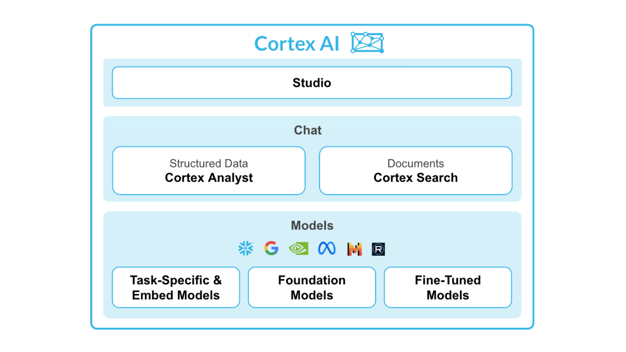
Source: Snowflake Cortex AI

Key features of Snowflake Cortex AI:

• Cortex Analyst: A self-serve analytics feature that enables users to interact with data using natural language.
• Cortex Search: Advanced, AI-based search system built for searching data within enterprise documents.
• LLMs and Embed Models: Connections to powerful LLMs like Snowflake Arctic, Meta Llama 3, and Mistral on a serverless architecture.
• Cortex Fine-Tuning: Enables custom small models to have the performance of LLMs without the high cost. 

Snowflake Cortex consists of two main parts—LLM functions and ML functions.

For LLM functions, you have:

1. Summarize
2. Translate
3. Complete
4. Extract Answer
5. Sentiment
6. Embed Text

We’ll look at each function in further detail later on below.

For ML functions, you have:

1. Anomaly detection: Automatically detects and alerts users to anomalies in their data.
2. Forecasting: Uses machine learning algorithms to make predictions based on historical data.
3. Classification: Classifies data into different categories or groups.
4. Top insights:  Identifies reasons for fluctuation in the values of metrics over a period of time.

Want to find out where to learn Snowflake and its functions? Our beginners’ Snowflake Tutorial and Snowflake certification guide will help you.

Why Use Snowflake Cortex AI with Python?

Let’s now look at the benefits of using these tools together.

Advantages of combining Snowflake Cortex AI with Python

Some key benefits of using Snowflake Cortex AI are:

• Python integration: It allows you to run Python ML models directly within Snowflake's computing environment.
• Model hosting: Models can be hosted and served for inference.
• No data movement: Since the models run within the Snowflake environment, there is no need to move large datasets to external servers.

Use cases and applications

Firstly, Snowflake Cortex AI is perfect for businesses looking to improve their data science capabilities without significant investment in resources. With its no-code environment, even non-technical users can easily develop and deploy ML models.

This is especially useful for smaller businesses or startups that may not have the budget to hire a team of data scientists or invest in expensive LLMs.

Secondly, by integrating Python into Snowflake's computing environment, users can take advantage of the vast library of available Python machine learning algorithms and tools. This means that they can create more advanced and accurate models without having to learn new programming languages.

Lastly, companies that have already adopted the Snowflake environment would reap the full benefits of Cortex AI as it seamlessly integrates with their existing data warehouse, eliminating the need for additional infrastructure or data migration.

With Snowflake Cortex AI, companies can easily and efficiently implement machine learning into their business processes. 

Getting Started With Snowflake Cortex AI

In this tutorial, we will walk through the process of setting up a machine learning pipeline using Python and Snowflake Cortex AI.

Prerequisites

Before you start working on ML with Snowflake Cortex AI, make sure you meet the following requirements:

Setting up a Snowflake account

First, you’ll need a Snowflake instance where your data is stored and processed. You can sign up on the Snowflake website.

In the sign-up form, fill in all your account details and take note to make the following selections on the second page. Select Standard edition for this tutorial and Amazon Web Services for the sake of simplicity and reproducibility. For the server, choose US West (Oregon) for the best selection of LLM functions available.

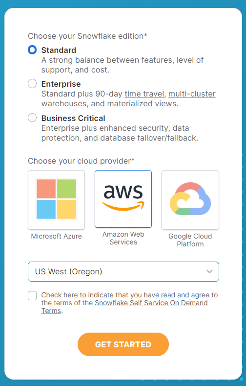
Once you have selected these options, click Get Started to receive the activation email. Head on over to your email to activate your account and your Snowflake account is ready to go.

Software requirements

Next up, you’ll also need to fulfill some other requirements for the software.

Here’s a simple list of things to have:

• Python Environment: Python 3.x with the necessary packages installed.
• Snowflake: Snowflake has to be installed from the terminal to connect your Python environment to your Snowflake account.
• VS Code: An integrated development environment (IDE) that’s suitable for Python can be used. Other alternatives include DataLab, Google Colab, or Jupyter Notebooks.

Before you begin any analysis, install all the relevant packages so your coding environment is ready.

To install the necessary packages, you can use pip:

pip install snowflake

pip install python-dotenv

After you’ve installed the libraries, you’ll need to set up your working folder and files to begin.

I’ve created a folder called Cortex AI Tutorial and included a new .env file containing the following information:

SNOWFLAKE_ACCOUNT = "<YOUR_ACCOUNT>" # eg. XXXX-XXXX

SNOWFLAKE_USER = "<YOUR_USER>" 

SNOWFLAKE_USER_PASSWORD = "<YOUR_PASSWORD>"

After entering your account information, save the file and create a Python or Jupyter Notebook file in the same folder.

Connecting to Snowflake

Now that you’re all set up, let’s get your Python environment connected to Snowflake.

To start with, open up your Python file and import all the necessary libraries. Here is the code to do so:

import os
from dotenv import load_dotenv
from snowflake.snowpark import Session
from snowflake.cortex import Summarize, Complete, ExtractAnswer, Sentiment, Translate, EmbedText768

Next, you’ll have to load up the variables you saved in the .env file you saved earlier. This will provide Snowflake with your account credentials to log in and use their functions.

# Loads environment variables from .env
load_dotenv()
connection_params = {
    "account": os.environ["SNOWFLAKE_ACCOUNT"],
    "user": os.environ["SNOWFLAKE_USER"],
    "password": os.environ["SNOWFLAKE_USER_PASSWORD"],
}

Once you’ve connected using the variables, you would need to set up a Snowflake session. This is the object that will handle all of your requests. 

# Creates a Snowflake session

snowflake_session = Session.builder.configs(connection_params).create()

Snowflake Cortex AI LLM Functions

The LLM functions within Cortex AI enable users to tap into the potential of LLMs without needing to develop their own AI models.

These functions help provide the average analytics user with AI-powered analysis through some basic tasks.

Here are the functions that Snowflake Cortex has:

1. SUMMARIZE

The summarize function is used to generate a summary of the data based on the input provided.

It uses LLMs to identify key information and present it in a condensed format.

For example, if you have a long text document and you want a quick overview of its contents, you can use the summarize function to get a brief summary that captures the important points. This saves time and allows for quicker analysis of large amounts of data.

Input language is currently limited to English at the time of writing this article.

See the code below for reference:

# Defines the Summarize LLM Function
def summarize(user_text):
    summary = Summarize(text=user_text, session=snowflake_session)
    return summary

2. TRANSLATE

The translate function is used to convert text from one language to another.

It makes use of machine learning algorithms and statistical models to accurately translate the text.

This can be useful when working with data or documents in different languages, as it allows for easier communication and understanding.

For example, if you have a report written in Spanish and need to present it to an English-speaking audience, you can use the translate function to quickly convert the text. This eliminates the need for manual translation and saves time.

See the code below for reference:

# Defines the Translate LLM Function
def translate(user_text):
    translation = Translate(
        text=user_text, from_language="en", to_language="ko", session=snowflake_session
    )
    return translation

3. COMPLETE

The complete function is an all-rounded function that can be used to carry out specific tasks. This is done through the use of sentence prompts that guide the AI model in providing the necessary information to execute a task.

See the code below for reference:

# Defines the Complete LLM Function
def complete(user_text):
    completion = Complete(
        model="snowflake-arctic",
        prompt=f"Provide 3 relevant keywords from the following text: {user_text}",
        session=snowflake_session,
    )
    return completion

4. EXTRACT_ANSWER

The extract answer function gives an answer based on the question provided to the model. The input must be in English in a string or JSON format.

See the code below for reference:

# Defines the Extract Answer LLM Function
def extract_answer(user_text):
    answer = ExtractAnswer(
        from_text=user_text,
        question="What are some reasons why young adult South Koreans love coffee?",
        session=snowflake_session,
    )
    return answer

5. SENTIMENT

The sentiment function provides a quantitative number based on the sentiment of the text provided. It outputs a value that ranges from -1 to 1. Values with -1 are the most negative 1 the most positive, and values around 0 are neutral.

See the code below for reference:

# Defines the Sentiment LLM Function
def sentiment(user_text):
    sentiment = Sentiment(text=user_text, session=snowflake_session)
    return sentiment

6. EMBED_TEXT

The embed text functions include the EMBED_TEXT_768 function and the EMBED_TEXT_1024 function. They create vector embeddings of 768 and 1024 dimensions respectively.

See the code below for reference on the EMBED_TEXT_768 functions:

# Defines the Embed Text LLM Function
def embed_text(user_text):
    embed_text = EmbedText768(text=user_text, model='snowflake-arctic-embed-m', session=snowflake_session)
    return embed_text

Now let’s put them all together in a main function and run it through a sample text to view the results.

I’ve used a simple, short piece of text to input into the model, as shown below:

For convenience of copying and pasting, here’s the text:

user_text = """
        Young adults in South Korea are embracing coffee as a blend of energy, comfort, and culture. 
        Coffee isn't just about staying awake during demanding studies or work; it’s a cherished part of daily routines. 
        With South Korea's bustling café culture, coffee shops have become popular spaces for socializing, studying, 
        or just taking a break from the fast-paced city life. 
        The diversity of flavors and trendy cafés also offers a unique, 
        stylish experience that fits right into the evolving lifestyle of young adults, 
        who seek both connection and personal moments in the midst of it all.
    """

Now, let’s run the code. It should take just a few seconds.

Here are the results:

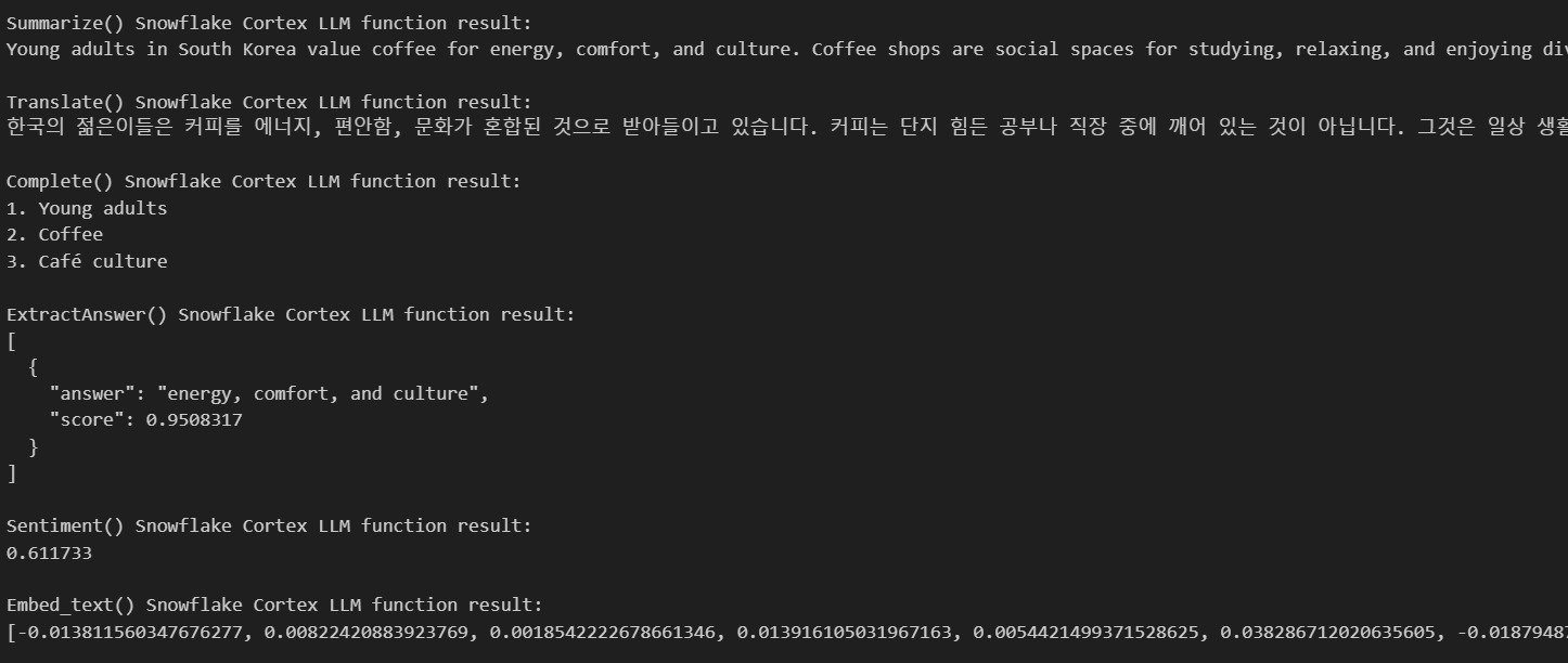
As you can see, the AI has given us all the results we need based on the text we’ve provided. It gave us a summary, translated my text into Korean, gave me three keywords based on my text, and provided some answers based on my questions.

Snowflake Cortex AI Machine Learning Functions

Cortex AI also has ML functions that can run using only SQL. Here are the several functions it provides.

1. Anomaly detection

Anomaly detection is essential for identifying unusual patterns that don't fit the expected behavior of your data. Snowflake simplifies anomaly detection by providing built-in machine learning functions based on a gradient boosting machine (GBM) that allows you to quickly identify outliers in your datasets.

Anomaly detection is particularly useful for tasks like:

• Detecting fraud in transaction data.
• Identifying unusual user behavior.
• Monitoring time series data for anomalies in system performance.

To perform anomaly detection, the Snowflake class ANOMALY_DETECTION (SNOWFLAKE.ML) can be used. This command creates an anomaly detection model object. This step fits your model to the training data.

Here is how you can use it:

CREATE [ OR REPLACE ] SNOWFLAKE.ML.ANOMALY_DETECTION <model_name>(
  INPUT_DATA => <reference_to_training_data>,
  [ SERIES_COLNAME => '<series_column_name>', ]
  TIMESTAMP_COLNAME => '<timestamp_column_name>',
  TARGET_COLNAME => '<target_column_name>',
  LABEL_COLNAME => '<label_column_name>',
  [ CONFIG_OBJECT => <config_object> ]
)
[ [ WITH ] TAG ( <tag_name> = '<tag_value>' [ , <tag_name> = '<tag_value>' , ... ] ) ]
[ COMMENT = '<string_literal>' ]

Once you’ve created the object, you can use the <model_name>!DETECT_ANOMALIES method to perform anomaly detection,

<model_name>!DETECT_ANOMALIES(
  INPUT_DATA => <reference_to_data_to_analyze>,
  TIMESTAMP_COLNAME => '<timestamp_column_name>',
  TARGET_COLNAME => '<target_column_name>',
  [ CONFIG_OBJECT => <configuration_object>, ]
  [ SERIES_COLNAME => '<series_column_name>' ]
)

This is the actual prediction step where the outliers will be detected using the method.

Here’s an example of how anomaly detection can be done using a dataset.

First, you can create a database by going to Data on the left tab, and then Add Data, followed by Load data into a Table.

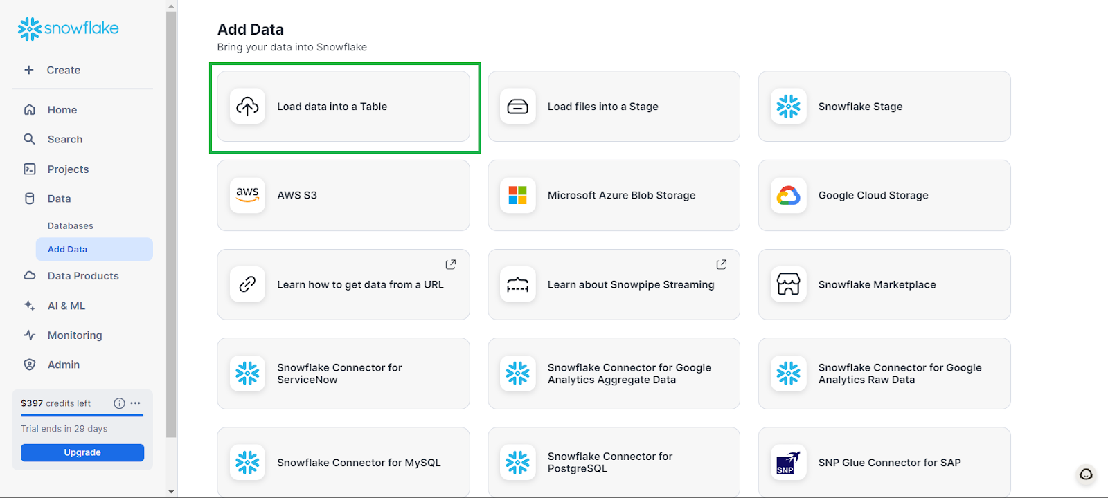
In the window that pops up, click on + Database and name your database. Click on Create, then in the main popup window, click on Cancel.

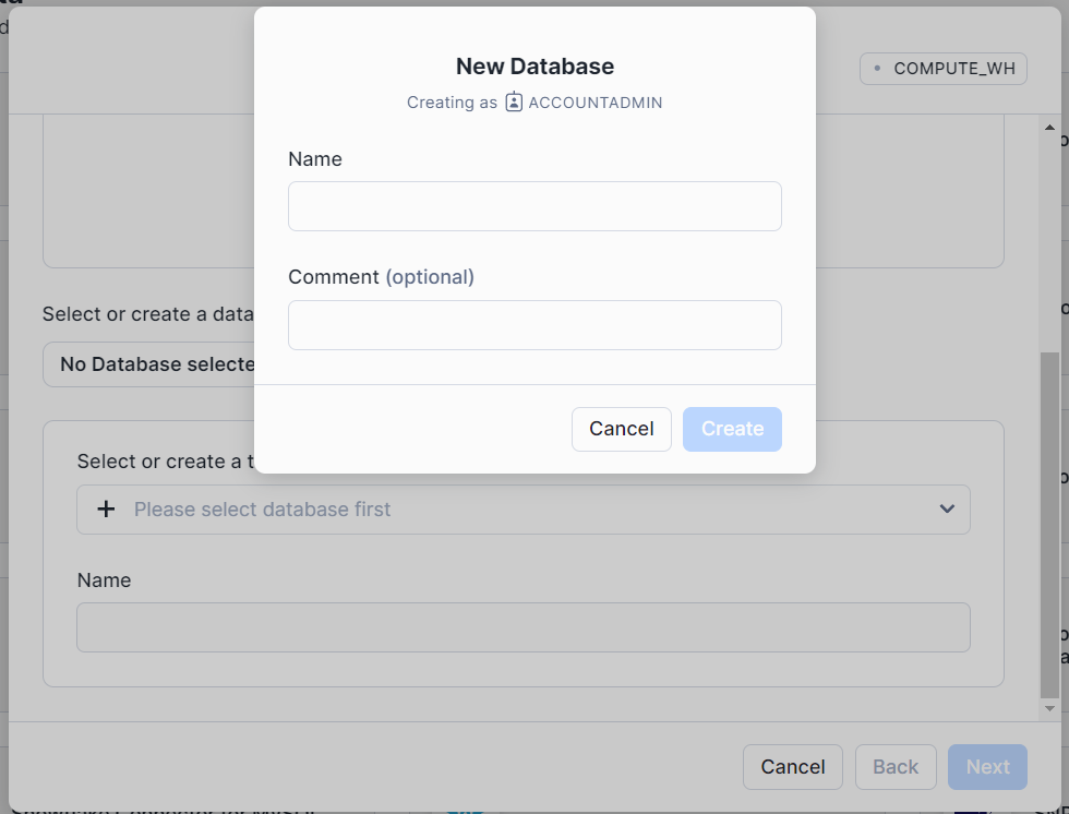
This will create an empty database that you can work with.

The examples below have been adapted from the Snowflake Documentation.

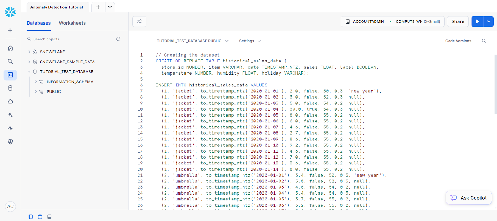
To begin the anomaly detection, go to a new SQL worksheet, select your new database as the data source, and paste the following code to create a table:

CREATE OR REPLACE TABLE historical_sales_data (

  store_id NUMBER, item VARCHAR, date TIMESTAMP_NTZ, sales FLOAT, label BOOLEAN,

  temperature NUMBER, humidity FLOAT, holiday VARCHAR);

// Creating the dataset
INSERT INTO historical_sales_data VALUES
  (1, 'jacket', to_timestamp_ntz('2020-01-01'), 2.0, false, 50, 0.3, 'new year'),
  (1, 'jacket', to_timestamp_ntz('2020-01-02'), 3.0, false, 52, 0.3, null),
  (1, 'jacket', to_timestamp_ntz('2020-01-03'), 5.0, false, 54, 0.2, null),
  (1, 'jacket', to_timestamp_ntz('2020-01-04'), 30.0, true, 54, 0.3, null),
  (1, 'jacket', to_timestamp_ntz('2020-01-05'), 8.0, false, 55, 0.2, null),
  (1, 'jacket', to_timestamp_ntz('2020-01-06'), 6.0, false, 55, 0.2, null),
  (1, 'jacket', to_timestamp_ntz('2020-01-07'), 4.6, false, 55, 0.2, null),
  (1, 'jacket', to_timestamp_ntz('2020-01-08'), 2.7, false, 55, 0.2, null),
  (1, 'jacket', to_timestamp_ntz('2020-01-09'), 8.6, false, 55, 0.2, null),
  (1, 'jacket', to_timestamp_ntz('2020-01-10'), 9.2, false, 55, 0.2, null),
  (1, 'jacket', to_timestamp_ntz('2020-01-11'), 4.6, false, 55, 0.2, null),
  (1, 'jacket', to_timestamp_ntz('2020-01-12'), 7.0, false, 55, 0.2, null),
  (1, 'jacket', to_timestamp_ntz('2020-01-13'), 3.6, false, 55, 0.2, null),
  (1, 'jacket', to_timestamp_ntz('2020-01-14'), 8.0, false, 55, 0.2, null),
  (2, 'umbrella', to_timestamp_ntz('2020-01-01'), 3.4, false, 50, 0.3, 'new year'),
  (2, 'umbrella', to_timestamp_ntz('2020-01-02'), 5.0, false, 52, 0.3, null),
  (2, 'umbrella', to_timestamp_ntz('2020-01-03'), 4.0, false, 54, 0.2, null),
  (2, 'umbrella', to_timestamp_ntz('2020-01-04'), 5.4, false, 54, 0.3, null),
  (2, 'umbrella', to_timestamp_ntz('2020-01-05'), 3.7, false, 55, 0.2, null),
  (2, 'umbrella', to_timestamp_ntz('2020-01-06'), 3.2, false, 55, 0.2, null),
  (2, 'umbrella', to_timestamp_ntz('2020-01-07'), 3.2, false, 55, 0.2, null),
  (2, 'umbrella', to_timestamp_ntz('2020-01-08'), 5.6, false, 55, 0.2, null),
  (2, 'umbrella', to_timestamp_ntz('2020-01-09'), 7.3, false, 55, 0.2, null),
  (2, 'umbrella', to_timestamp_ntz('2020-01-10'), 8.2, false, 55, 0.2, null),
  (2, 'umbrella', to_timestamp_ntz('2020-01-11'), 3.7, false, 55, 0.2, null),
  (2, 'umbrella', to_timestamp_ntz('2020-01-12'), 5.7, false, 55, 0.2, null),
  (2, 'umbrella', to_timestamp_ntz('2020-01-13'), 6.3, false, 55, 0.2, null),
  (2, 'umbrella', to_timestamp_ntz('2020-01-14'), 2.9, false, 55, 0.2, null);

Your code should go into an SQL worksheet that looks like this:

This is followed by the following statements to create a table named new_sales_data.

// Creating a new table and adding training data
CREATE OR REPLACE TABLE new_sales_data (
  store_id NUMBER, item VARCHAR, date TIMESTAMP_NTZ, sales FLOAT,
  temperature NUMBER, humidity FLOAT, holiday VARCHAR);
INSERT INTO new_sales_data VALUES
  (1, 'jacket', to_timestamp_ntz('2020-01-16'), 6.0, 52, 0.3, null),
  (1, 'jacket', to_timestamp_ntz('2020-01-17'), 20.0, 53, 0.3, null),
  (2, 'umbrella', to_timestamp_ntz('2020-01-16'), 3.0, 52, 0.3, null),
  (2, 'umbrella', to_timestamp_ntz('2020-01-17'), 70.0, 53, 0.3, null);

Now, create the anomaly detection model:

// Creating anomaly detection model object
CREATE OR REPLACE VIEW view_with_training_data
  AS SELECT date, sales FROM historical_sales_data
    WHERE store_id=1 AND item='jacket';
CREATE OR REPLACE SNOWFLAKE.ML.ANOMALY_DETECTION basic_model(
  INPUT_DATA => TABLE(view_with_training_data),
  TIMESTAMP_COLNAME => 'date',
  TARGET_COLNAME => 'sales',
  LABEL_COLNAME => '');

This should create a result stating that a model has been created as shown below.

Next, let’s use the object model to do some detection.

// Perform anomaly detection
CREATE OR REPLACE VIEW view_with_data_to_analyze
  AS SELECT date, sales FROM new_sales_data
    WHERE store_id=1 and item='jacket';
CALL basic_model!DETECT_ANOMALIES(
  INPUT_DATA => TABLE(view_with_data_to_analyze),
  TIMESTAMP_COLNAME =>'date',
  TARGET_COLNAME => 'sales'
);

Here’s the output of the detection:

2. Classification

Classification involves categorizing data into predefined classes. With Snowflake, you can classify data directly from within Snowflake, eliminating the need for data export to external ML environments. 

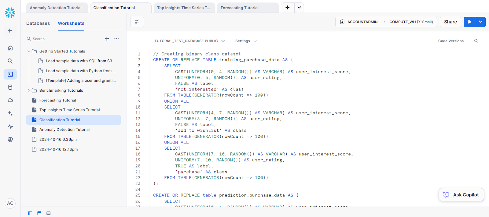
To begin, create a sample dataset using the following code:

// Creating binary class dataset
CREATE OR REPLACE TABLE training_purchase_data AS (
    SELECT
        CAST(UNIFORM(0, 4, RANDOM()) AS VARCHAR) AS user_interest_score,
        UNIFORM(0, 3, RANDOM()) AS user_rating,
        FALSE AS label,
        'not_interested' AS class
    FROM TABLE(GENERATOR(rowCount => 100))
    UNION ALL
    SELECT
        CAST(UNIFORM(4, 7, RANDOM()) AS VARCHAR) AS user_interest_score,
        UNIFORM(3, 7, RANDOM()) AS user_rating,
        FALSE AS label,
        'add_to_wishlist' AS class
    FROM TABLE(GENERATOR(rowCount => 100))
    UNION ALL
    SELECT
        CAST(UNIFORM(7, 10, RANDOM()) AS VARCHAR) AS user_interest_score,
        UNIFORM(7, 10, RANDOM()) AS user_rating,
        TRUE AS label,
        'purchase' AS class
    FROM TABLE(GENERATOR(rowCount => 100))
);
CREATE OR REPLACE table prediction_purchase_data AS (
    SELECT
        CAST(UNIFORM(0, 4, RANDOM()) AS VARCHAR) AS user_interest_score,
        UNIFORM(0, 3, RANDOM()) AS user_rating
    FROM TABLE(GENERATOR(rowCount => 100))
    UNION ALL
    SELECT
        CAST(UNIFORM(4, 7, RANDOM()) AS VARCHAR) AS user_interest_score,
        UNIFORM(3, 7, RANDOM()) AS user_rating
    FROM TABLE(GENERATOR(rowCount => 100))
    UNION ALL
    SELECT
        CAST(UNIFORM(7, 10, RANDOM()) AS VARCHAR) AS user_interest_score,
        UNIFORM(7, 10, RANDOM()) AS user_rating
    FROM TABLE(GENERATOR(rowCount => 100))
);

For the purposes of training data, let’s create a new view.

// Creating view for training data
CREATE OR REPLACE view binary_classification_view AS
    SELECT user_interest_score, user_rating, label
FROM training_purchase_data;
SELECT * FROM binary_classification_view ORDER BY RANDOM(42) LIMIT 5;

This view should output the following results:

Next, let’s train the model based on our training data:

// Training a binary classification model
CREATE OR REPLACE SNOWFLAKE.ML.CLASSIFICATION model_binary(
    INPUT_DATA => SYSTEM$REFERENCE('view', 'binary_classification_view'),
    TARGET_COLNAME => 'label'
);

To perform classification, use the PREDICT method:

// Performing prediction using PREDICT method
SELECT model_binary!PREDICT(INPUT_DATA => {*})
    AS prediction FROM prediction_purchase_data;

Here’s what the prediction looks like:

To format it nicely, use this SQL statement:

// Formatting SQL predictions
SELECT *, model_binary!PREDICT(INPUT_DATA => {*})
    AS predictions FROM prediction_purchase_data;

You should arrive at this neat output format for the predictions:

3. Top insights

Top Insights is a monitoring tool to look for fluctuations in your metrics over time through a time-series analysis. Using a decision tree model,  Top Insights can identify the most significant contributing factors to an increase or decrease in a particular metric.

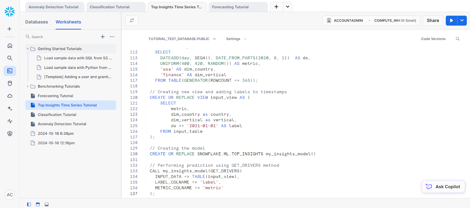
Let’s look at an example of a time-series analysis using this function.

Firstly, let’s create a dataset:

// Creating dataset
CREATE OR REPLACE TABLE input_table(
  ds DATE, metric NUMBER, dim_country VARCHAR, dim_vertical VARCHAR);
INSERT INTO input_table
  SELECT
    DATEADD(day, SEQ4(), DATE_FROM_PARTS(2020, 4, 1)) AS ds,
    UNIFORM(1, 10, RANDOM()) AS metric,
    'usa' AS dim_country,
    'tech' AS dim_vertical
  FROM TABLE(GENERATOR(ROWCOUNT => 365));
INSERT INTO input_table
  SELECT
    DATEADD(day, SEQ4(), DATE_FROM_PARTS(2020, 4, 1)) AS ds,
    UNIFORM(1, 10, RANDOM()) AS metric,
    'usa' AS dim_country,
    'auto' AS dim_vertical
  FROM TABLE(GENERATOR(ROWCOUNT => 365));
INSERT INTO input_table
  SELECT
    DATEADD(day, seq4(), DATE_FROM_PARTS(2020, 4, 1)) AS ds,
    UNIFORM(1, 10, RANDOM()) AS metric,
    'usa' AS dim_country,
    'fashion' AS dim_vertical
  FROM TABLE(GENERATOR(ROWCOUNT => 365));
INSERT INTO input_table
  SELECT
    DATEADD(day, SEQ4(), DATE_FROM_PARTS(2020, 4, 1)) AS ds,
    UNIFORM(1, 10, RANDOM()) AS metric,
    'usa' AS dim_country,
    'finance' AS dim_vertical
  FROM TABLE(GENERATOR(ROWCOUNT => 365));
INSERT INTO input_table
  SELECT
    DATEADD(day, SEQ4(), DATE_FROM_PARTS(2020, 4, 1)) AS ds,
    UNIFORM(1, 10, RANDOM()) AS metric,
    'canada' AS dim_country,
    'fashion' AS dim_vertical
  FROM TABLE(GENERATOR(ROWCOUNT => 365));
INSERT INTO input_table
  SELECT
    DATEADD(day, SEQ4(), DATE_FROM_PARTS(2020, 4, 1)) AS ds,
    UNIFORM(1, 10, RANDOM()) AS metric,
    'canada' AS dim_country,
    'finance' AS dim_vertical
  FROM TABLE(GENERATOR(ROWCOUNT => 365));
INSERT INTO input_table
  SELECT
    DATEADD(day, SEQ4(), DATE_FROM_PARTS(2020, 4, 1)) AS ds,
    UNIFORM(1, 10, RANDOM()) AS metric,
    'canada' AS dim_country,
    'tech' AS dim_vertical
  FROM TABLE(GENERATOR(ROWCOUNT => 365));
INSERT INTO input_table
  SELECT
    DATEADD(day, SEQ4(), DATE_FROM_PARTS(2020, 4, 1)) AS ds,
    UNIFORM(1, 10, RANDOM()) AS metric,
    'canada' AS dim_country,
    'auto' AS dim_vertical
  FROM TABLE(GENERATOR(ROWCOUNT => 365));
INSERT INTO input_table
  SELECT
    DATEADD(day, SEQ4(), DATE_FROM_PARTS(2020, 4, 1)) AS ds,
    UNIFORM(1, 10, RANDOM()) AS metric,
    'france' AS dim_country,
    'fashion' AS dim_vertical
  FROM TABLE(GENERATOR(ROWCOUNT => 365));
INSERT INTO input_table
  SELECT
    DATEADD(day, SEQ4(), DATE_FROM_PARTS(2020, 4, 1)) AS ds,
    UNIFORM(1, 10, RANDOM()) AS metric,
    'france' AS dim_country,
    'finance' AS dim_vertical
  FROM TABLE(GENERATOR(ROWCOUNT => 365));
INSERT INTO input_table
  SELECT
    DATEADD(day, SEQ4(), DATE_FROM_PARTS(2020, 4, 1)) AS ds,
    UNIFORM(1, 10, RANDOM()) AS metric,
    'france' AS dim_country,
    'tech' AS dim_vertical
  FROM TABLE(GENERATOR(ROWCOUNT => 365));
INSERT INTO input_table
  SELECT
    DATEADD(day, SEQ4(), DATE_FROM_PARTS(2020, 4, 1)) AS ds,
    UNIFORM(1, 10, RANDOM()) AS metric,
    'france' AS dim_country,
    'auto' AS dim_vertical
  FROM TABLE(GENERATOR(ROWCOUNT => 365));
-- Data for the test group
INSERT INTO input_table
  SELECT
    DATEADD(day, SEQ4(), DATE_FROM_PARTS(2020, 8, 1)) AS ds,
    UNIFORM(300, 320, RANDOM()) AS metric,
    'usa' AS dim_country,
    'auto' AS dim_vertica
  FROM TABLE(GENERATOR(ROWCOUNT => 365));
INSERT INTO input_table
  SELECT
    DATEADD(day, SEQ4(), DATE_FROM_PARTS(2020, 8, 1))  AS ds,
    UNIFORM(400, 420, RANDOM()) AS metric,
    'usa' AS dim_country,
    'finance' AS dim_vertical
  FROM TABLE(GENERATOR(ROWCOUNT => 365));
// Creating new view and adding labels to timestamps
CREATE OR REPLACE VIEW input_view AS (
    SELECT
        metric,
        dim_country as country,
        dim_vertical as vertical,
        ds >= '2021-01-01' AS label
    FROM input_table
);

Next, we have to create the model object for the prediction. This is needed to access the GET_DRIVERS method.

// Creating the model
CREATE OR REPLACE SNOWFLAKE.ML.TOP_INSIGHTS my_insights_model()

Lastly, for the prediction, call the GET_DRIVERS method.

// Performing prediction using GET_DRIVERS method
CALL my_insights_model!GET_DRIVERS(
  INPUT_DATA => TABLE(input_view),
  LABEL_COLNAME => 'label',
  METRIC_COLNAME => 'metric'
);

This should give you the following results:

4. Forecasting

Forecasting is crucial when you need to predict future values based on historical data. Whether it's sales forecasting, predicting energy consumption, or forecasting web traffic, Snowflake’s built-in functions make these tasks much simpler.

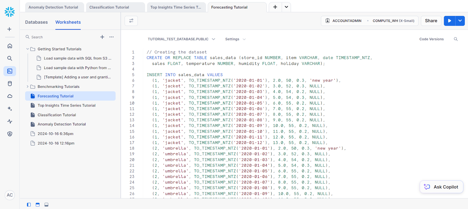
For our example, let’s look at doing some forecasting on a single series:

// Creating the dataset
CREATE OR REPLACE TABLE sales_data (store_id NUMBER, item VARCHAR, date TIMESTAMP_NTZ,
  sales FLOAT, temperature NUMBER, humidity FLOAT, holiday VARCHAR);
INSERT INTO sales_data VALUES
  (1, 'jacket', TO_TIMESTAMP_NTZ('2020-01-01'), 2.0, 50, 0.3, 'new year'),
  (1, 'jacket', TO_TIMESTAMP_NTZ('2020-01-02'), 3.0, 52, 0.3, NULL),
  (1, 'jacket', TO_TIMESTAMP_NTZ('2020-01-03'), 4.0, 54, 0.2, NULL),
  (1, 'jacket', TO_TIMESTAMP_NTZ('2020-01-04'), 5.0, 54, 0.3, NULL),
  (1, 'jacket', TO_TIMESTAMP_NTZ('2020-01-05'), 6.0, 55, 0.2, NULL),
  (1, 'jacket', TO_TIMESTAMP_NTZ('2020-01-06'), 7.0, 55, 0.2, NULL),
  (1, 'jacket', TO_TIMESTAMP_NTZ('2020-01-07'), 8.0, 55, 0.2, NULL),
  (1, 'jacket', TO_TIMESTAMP_NTZ('2020-01-08'), 9.0, 55, 0.2, NULL),
  (1, 'jacket', TO_TIMESTAMP_NTZ('2020-01-09'), 10.0, 55, 0.2, NULL),
  (1, 'jacket', TO_TIMESTAMP_NTZ('2020-01-10'), 11.0, 55, 0.2, NULL),
  (1, 'jacket', TO_TIMESTAMP_NTZ('2020-01-11'), 12.0, 55, 0.2, NULL),
  (1, 'jacket', TO_TIMESTAMP_NTZ('2020-01-12'), 13.0, 55, 0.2, NULL),
  (2, 'umbrella', TO_TIMESTAMP_NTZ('2020-01-01'), 2.0, 50, 0.3, 'new year'),
  (2, 'umbrella', TO_TIMESTAMP_NTZ('2020-01-02'), 3.0, 52, 0.3, NULL),
  (2, 'umbrella', TO_TIMESTAMP_NTZ('2020-01-03'), 4.0, 54, 0.2, NULL),
  (2, 'umbrella', TO_TIMESTAMP_NTZ('2020-01-04'), 5.0, 54, 0.3, NULL),
  (2, 'umbrella', TO_TIMESTAMP_NTZ('2020-01-05'), 6.0, 55, 0.2, NULL),
  (2, 'umbrella', TO_TIMESTAMP_NTZ('2020-01-06'), 7.0, 55, 0.2, NULL),
  (2, 'umbrella', TO_TIMESTAMP_NTZ('2020-01-07'), 8.0, 55, 0.2, NULL),
  (2, 'umbrella', TO_TIMESTAMP_NTZ('2020-01-08'), 9.0, 55, 0.2, NULL),
  (2, 'umbrella', TO_TIMESTAMP_NTZ('2020-01-09'), 10.0, 55, 0.2, NULL),
  (2, 'umbrella', TO_TIMESTAMP_NTZ('2020-01-10'), 11.0, 55, 0.2, NULL),
  (2, 'umbrella', TO_TIMESTAMP_NTZ('2020-01-11'), 12.0, 55, 0.2, NULL),
  (2, 'umbrella', TO_TIMESTAMP_NTZ('2020-01-12'), 13.0, 55, 0.2, NULL);
-- Future values for additional columns (features)
CREATE OR REPLACE TABLE future_features (store_id NUMBER, item VARCHAR,
  date TIMESTAMP_NTZ, temperature NUMBER, humidity FLOAT, holiday VARCHAR);
INSERT INTO future_features VALUES
  (1, 'jacket', TO_TIMESTAMP_NTZ('2020-01-13'), 52, 0.3, NULL),
  (1, 'jacket', TO_TIMESTAMP_NTZ('2020-01-14'), 53, 0.3, NULL),
  (2, 'umbrella', TO_TIMESTAMP_NTZ('2020-01-13'), 52, 0.3, NULL),
  (2, 'umbrella', TO_TIMESTAMP_NTZ('2020-01-14'), 53, 0.3, NULL);

Next, let’s separate the training data from the dataset.

// Creating a view for training data
CREATE OR REPLACE VIEW v1 AS SELECT date, sales
  FROM sales_data WHERE store_id=1 AND item='jacket';
SELECT * FROM v1;

Before you can start your forecasting, you’ll need to train up your model based on the training data you’ve selected.

Here’s how you can do it:

// Training a forecasting model
CREATE SNOWFLAKE.ML.FORECAST model1(
  INPUT_DATA => TABLE(v1),
  TIMESTAMP_COLNAME => 'date',
  TARGET_COLNAME => 'sales'
);

Lastly, for the forecast, you can call the FORECAST method to do the prediction step.

// Performing the forecast by calling the FORECAST method
call model1!FORECAST(FORECASTING_PERIODS => 5);

This is the resulting output of our forecasting.

Monitoring ML Models in Snowflake

Monitoring model performance can be done by creating dashboards in Snowflake using third-party integrations (like Tableau) or querying Snowflake logs. Some useful metrics like accuracy, precision, and recall can be used for tracking models.

Conclusion

Snowflake Cortex AI simplifies machine learning by enabling seamless integration of models from the Snowflake platform. This tutorial walked you through using Snowflake Cortex AI and Snowflake Cortex ML functions.

This solution leverages the scalability of Snowflake and the flexibility of Python, making it ideal for organizations that want to implement machine learning without moving data outside the cloud.

Looking for more resources on Snowflake? You’ll like our Snowflake Beginner Tutorial and our Snowpark guide. If you’re looking for something more comprehensive, then the Introduction to Snowflake course might be the right course for you.