Excel Transpose Guide: Convert Rows to Columns & Vice Versa

Transposing data in Excel allows you to flip your data orientation, turning rows into columns and columns into rows. This technique is particularly useful when you need to restructure your dataset for better analysis, visualization, or reporting.

Whether you're preparing data for a PivotTable, creating a summary view, or simply need to change your data layout, Excel offers three main methods to transpose your data:

1. Paste Special - A quick one-time conversion

2. TRANSPOSE() function - A dynamic formula-based approach

3. Power Query - An advanced method for larger datasets

In this article, you'll learn step-by-step how to use each method, when to apply them, and important considerations to keep in mind. If you are new to Excel, we invite you to explore our Data Analysis in Excel course, where you can learn about basic operations such as PivotTables and logical functions. 

Quick Answer

Although Excel offers several ways to transpose data as mentioned in the introduction, the quickest way is to use Paste Special:

• Select and copy your data (Ctrl + C).

• Right-click on the destination cell where you want the transposed data to appear.

• Select "Paste Special."

• Check the "Transpose" box.

• Click OK.

This immediately flips your rows to columns and columns to rows, providing a fast solution for most transposing needs.

What Does Transpose Mean in Excel?

Transposing in Excel means converting rows into columns and columns into rows. It's essentially rotating your data by 90 degrees, changing its orientation while preserving all the information.

When you transpose data, the first row becomes the first column, the second row becomes the second column, and so on.

For example, if you have a dataset with product names in rows and monthly sales in columns, transposing would give you product names in columns and monthly sales in rows.

Ways to Transpose in Excel

Excel offers three distinct methods to transpose data, each with its own advantages and ideal use cases. Let's explore each technique step-by-step to help you choose the right approach.

1. Using paste special to transpose data

The Paste Special method is the simplest way to transpose data in Excel. It creates a one-time copy of your data in the transposed orientation. Let's walk through an example. Imagine we have the following regional sales data in vertical format: 

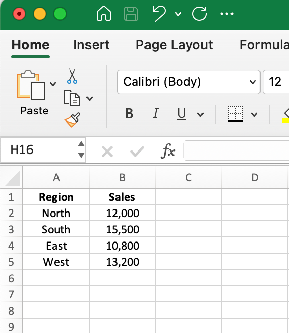
Example of Original Data in Vertical Format. Image by Author. 

To transpose this data from a vertical to horizontal layout:

1. Select all the data you want to transpose (in this case, cells A1:B5).
2. Copy the data (Ctrl+C or right-click and select Copy).
3. Click on the cell where you want the transposed data to appear (such as cell D1).
4. Right-click and select Paste Special from the context menu.

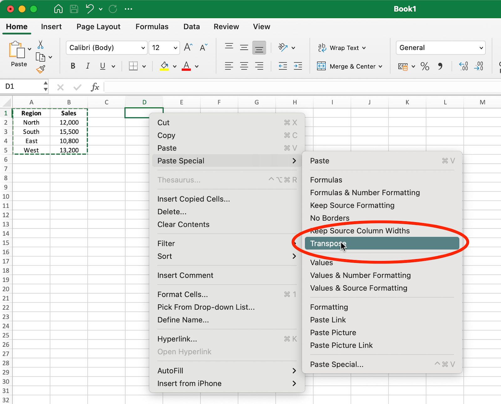
The Paste Special method and Transpose Option. Image by Author. 

5. In the Paste Special dialog box, check the Transpose box and click OK.

The result after transposing is shown below:

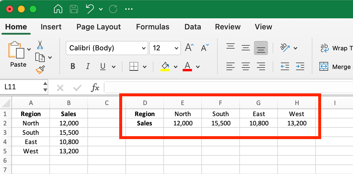
Result after Transposing the Original Data. Image by Author. 

Notice how the data has been completely rotated - what was previously in rows is now in columns, and vice versa. The region names that were in column A are now across row 1, and the sales figures that were in column B are now across row 2.

When to use this method:

• For quick, one-time data transformations
• When you need a simple solution that doesn't require formulas
• For smaller datasets that won't need frequent updating

Advantages: Simple and quick to apply with just a few clicks. 

Limitations: Creates a static copy that doesn't update if your original data changes.

2. Using the TRANSPOSE() function

The TRANSPOSE() function offers a dynamic alternative to Paste Special. Unlike the previous method that creates a static copy, this function maintains a live link to your original data, automatically updating the transposed results whenever the source data changes.

Let's use the same regional sales data to demonstrate how this works:

1. First, you need to select the destination range where your transposed data will appear. For our regional sales data example, we need to select cells that will accommodate our transposed structure. Since the original data is 5 rows by 2 columns, we'll need to select a range that is 2 rows by 5 columns.

2. With your destination cells in focus, enter the TRANSPOSE() formula in the formula bar:

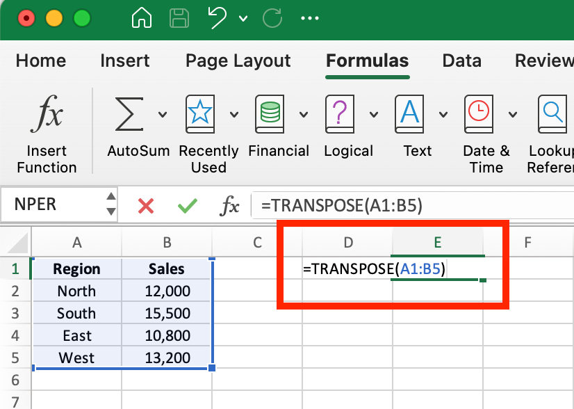
The TRANSPOSE() Function in Excel. Image by Author. 

3. In modern Excel (2019 or Microsoft 365), simply press Enter. For older Excel versions, you'll need to press Ctrl+Shift+Enter, as this is an array formula.

The result will look similar to our previous example, but with an important difference: if you change any value in the original data, the transposed version will automatically update to reflect those changes.

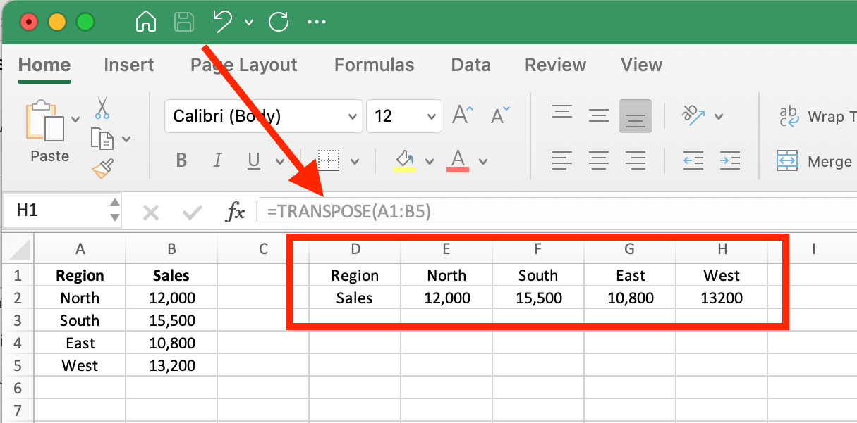
Result after using TRANSPOSE() Function. Image by Author. 

When to use this method:

• When your source data changes frequently
• When you need to maintain a live connection between original and transposed data
• For creating dynamic reports or dashboards that need to refresh automatically

Advantages: Creates a dynamic link that updates automatically when source data changes. 

Limitations: Requires careful selection of the correct destination range size; requires understanding of array formulas for older Excel versions.

3. Using Power Query to transpose data

Power Query is Excel's most powerful data transformation tool, perfect for handling larger datasets and complex transformations. While it requires more steps than the previous methods, it offers unmatched flexibility.

Let's use our same regional sales data to demonstrate how Power Query can transpose data:

1. Start by clicking on the Data tab in the Excel ribbon, then select the Get Data (Power Query) option.

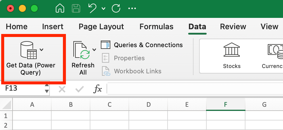
How to start Power Query in Excel. Image by Author. 

2. In the dialog box that appears, you'll see various data source options. Since we're working with a small example that's already in Excel, select Blank table which allows us to manually enter our data. Keep in mind, however, that the versatility of data sources available to Power Query is one of its core advantages.

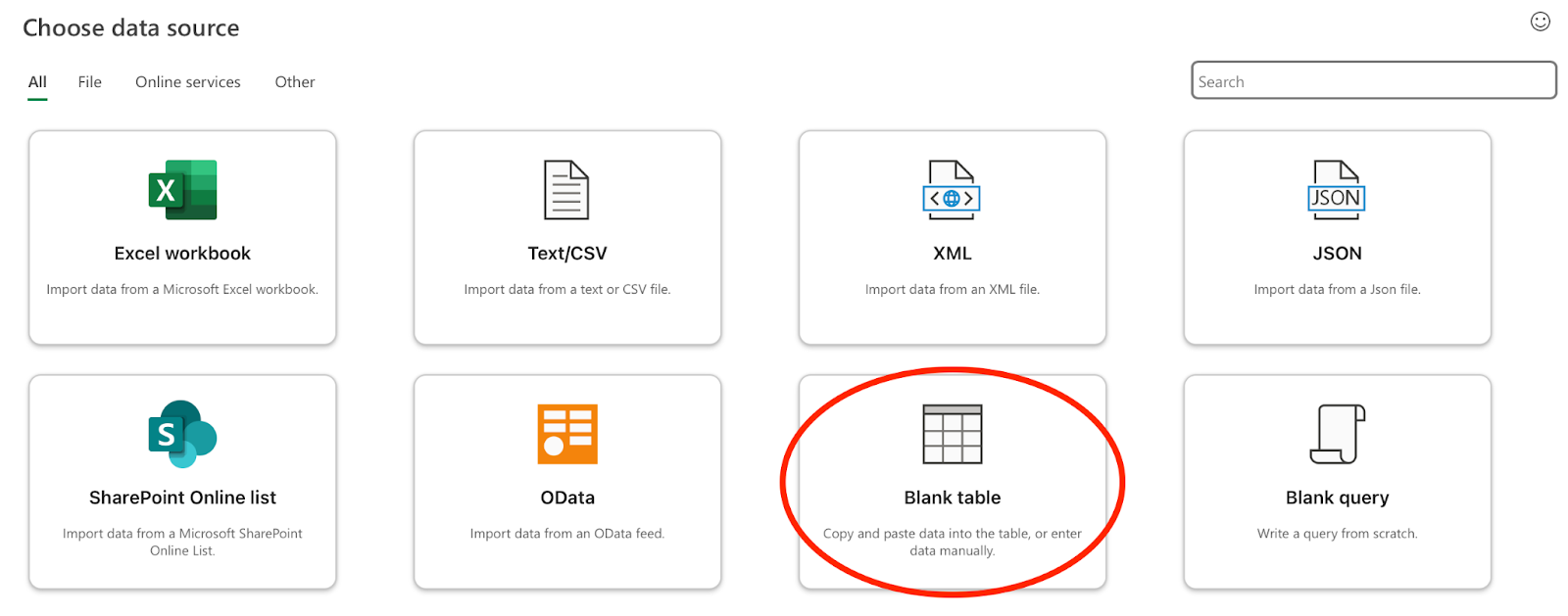
Opting for Blank Table Option for the Data Source. Image by Author. 

3. In the next screen, enter your data (or paste it from your worksheet) into the table. Make sure to check Use first row as headers if your data includes column headers.

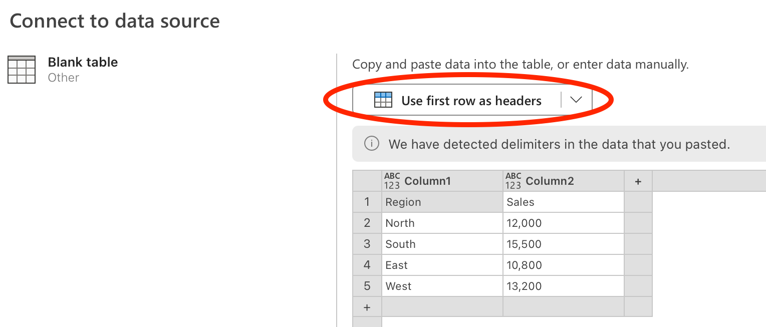
Entering Data for Power Query. Image by Author. 

4. After you click on Next, it will open the Power Query Editor with your data loaded. Now, click on the Transform tab in the ribbon, and select Transpose from the menu options.

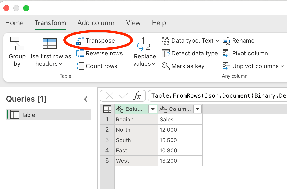
Transforming Data via the Transpose Feature in Power Query. Image by Author. 

5. You'll immediately see your data transposed in the preview window. Notice how Power Query automatically flips your rows and columns. The formula bar shows Table.Transpose(Source) indicating the transformation being applied.

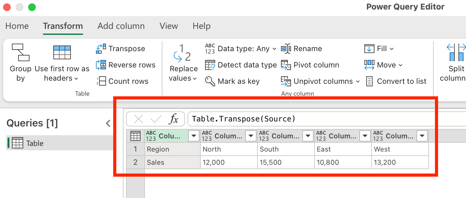
Result of Transpose in Power Query. Image by Author. 

6. Once you're satisfied with the transformation, click Close & Load from the Home tab to send the transposed data back to your Excel worksheet.

When to use this method:

• For large datasets where the other methods might be cumbersome
• When you need to perform additional transformations beyond just transposing
• As part of a more complex data cleaning and preparation workflow
• For repetitive tasks that you want to automate

Advantages:

• Ideal for large datasets and complex data transformations
• Creates a query that can be refreshed when source data changes
• Offers additional data cleaning options in the same workflow
• Can be saved as part of a repeatable process

Limitations:

• Requires more steps than the other methods
• Has a steeper learning curve for beginners
• Opens a separate editor window

Transposing Columns, Rows, and Tables

While we've explored the three main methods for transposing data in Excel, let's briefly address some specific scenarios you might encounter.

How to transpose columns to rows in Excel

When you have data organized in columns and need it in rows, use any of the methods we've discussed:

Using Paste Special:

1. Select and copy your column-based data (Ctrl + C).
2. Right-click on the first cell of the new row where you want the data to appear.
3. Click Paste Special, check Transpose.
4. Click OK to see your columns flipped into rows.

This instantly rearranges the data but creates a static copy.

Using the TRANSPOSE() Function:

1. Select an empty range that matches the number of rows in the original columns.

2. Type =TRANSPOSE(A1:A5) (modify as needed).

3. Press Enter (or Ctrl + Shift + Enter in older versions).

This keeps the transposed data connected to the original columns, ensuring it updates automatically.

How to transpose rows to columns in Excel

If your data is structured in rows but needs to be displayed in columns, you can use Excel's Paste Special feature for a quick one-time conversion or the TRANSPOSE() function for a dynamic approach.

Using Paste Special:

1. Select and copy your row-based data (Ctrl + C).
2. Right-click on the destination cell where you want the columns to appear.
3. Click Paste Special and check the Transpose box.
4. Click OK to see your rows flipped into columns.

Notice that the steps are the exact same for how to transpose columns into rows. Excel sees rows and columns as interchangeable.

Using the TRANSPOSE() function:

1. Select an empty range with the same number of columns as your original rows.

2. Type =TRANSPOSE(A1:F1) (adjust the range as needed).

3. Press Enter or Ctrl + Shift + Enter  .

Now, any changes in the original row will automatically update in the transposed columns.

If you're working with larger datasets that require frequent updates, Power Query is another effective way to automate column-to-row or row-to-column transformations while keeping the data linked. In the earlier section, I included the steps for how to use Power Query for transposing. 

How to transpose tables in Excel

When working with entire tables or structured ranges:

1. For smaller tables, simply select the entire range and use Paste Special → Transpose, as I showed in the earlier sections.
2. For larger tables with many columns and rows, Power Query provides more control and can handle any table size efficiently.
3. For tables where only a portion needs transposing, you may need to split your approach—transposing certain sections while keeping others in their original orientation

Remember that transposing a table will switch not just your data but also your headers. In many cases, you'll want your first row to become your first column (and vice versa) to maintain proper data labeling.

Additional Things to Consider

When transposing data in Excel, there are a few important considerations that can help you avoid common issues and enhance your workflow:

Handling blank cells

The TRANSPOSE() function may replace blanks with zeros, which isn't always desirable. To retain blank values when using this function, you can use a nested IF() statement:

=TRANSPOSE(IF(A1:F5="","",A1:F5))	

This formula checks if cells in the original range are empty and, if so, keeps them empty in the transposed result rather than converting them to zeros.

Maintaining links to source data

As we've discussed, the three transposition methods handle links to source data differently:

• Paste Special creates a static copy with no connection to the original data.

• The TRANSPOSE() function maintains a dynamic link, automatically updating when source data changes.

• Power Query allows you to refresh the connection when needed, giving you control over when updates occur.

Choose the appropriate method based on how frequently your source data changes and whether you need automatic updates.

Using TRANSPOSE() with conditional formatting

When using the TRANSPOSE() function, be aware that formatting does not carry over. If your original data uses conditional formatting to highlight important values, you'll need to apply new conditional formatting rules to the transposed range.

This applies to all visual formatting, including cell colors, fonts, and borders. Only the values themselves are transposed, not their visual presentation.

Conclusion

Transposing data in Excel is a valuable skill that can significantly improve your data organization and analysis workflows. Each of the three methods we've explored offers distinct advantages depending on your specific needs.

For more advanced data manipulation techniques in Excel, consider exploring our Excel Fundamentals skill track, which covers a range of skills to enhance your data analysis capabilities. If you're interested in expanding your data transformation skills beyond Excel, check out our tutorial on How to Transpose a Matrix in R for similar techniques in the R programming environment.