Course
Introduction to R
4 hr
3M
In this tutorial, you will be familiar with the Bioconductor space. By this, you will be able to perform computational and statistical analysis on the results of your biological experiment, as it is necessary for any researcher to prove the significance of their conclusions. In other words, you will be capable of manifesting whether the used data are consistent with your hypothesis by using this project. Besides, you can validate your scientific question statistically without wasting too much time and money.
In brief, this tutorial will straighten out:
- What is Bioconductor?
- What do Bioconductor R Packages stand for?
- How can we use it?
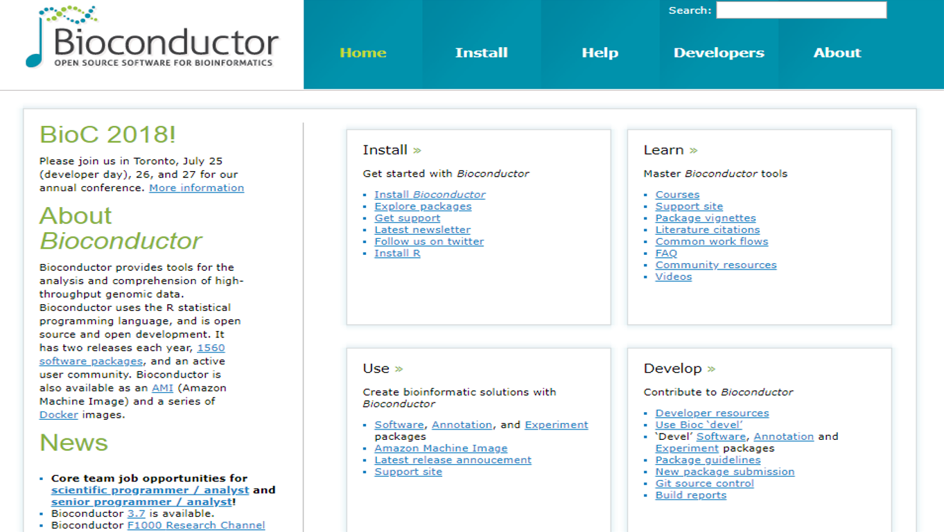
Bioconductor is an open software development for computational biology and bioinformatics. This is an open-source, open-development software project for the computational biology community. It’s open-source because anybody can read and modify the underlying code, and open-development because anybody can contribute and participate in the development of the code. It speaks the R language which is a widely used language for data science since it is a flexible language, especially for data analysis. R also has high-quality graphics, and it can easily be a bad tool for other languages. Bioconductor provides access to powerful statistical and graphical methods for the analysis of genomic data. It also facilitates the integration of biological metadata like GenBank, GO, LocusLink and PubMed in the analysis of experimental data.
Furthermore, it allows the rapid development of extensible, interoperable, and scalable software. Also, high-quality documentation and reproducible research can be promoted using Bioconductor. This prepares training in computational and statistical methods. Briefly, Bioconductor can be separated into three different parts as below:
| Statistical Analysis | Comprehension | High-throughput |
|---|---|---|
| Large data | Biological context | Sequencing |
| Technological artifacts | Visualization | Microarrays |
| Designed experiments | Reproducibility | Flow cytometry |
Analysis in computational biology almost always needs lots of different tools to put them together in order to answer a specific question. That will usually turn to be a package to be used by the other researchers, too. So, Bioconductor is additionally a software repository of R packages with some rules and guiding principles. Version 3.7 has more than 1500 packages. These are used by thousands of researchers around the world. These packages generally have excellent documentation. As everyone can contribute, there can be multiple choices of packages to solve a specific problem. So, this creates a competitive environment among package developers.
The website includes materials on how to install, learn, use and contribute back to Bioconductor projects. The project was started in the Fall of 2001 and includes more than 20 core developers in the US, Europe, and Australia.
Concisely, Bioconductor works on statistical analysis and comprehension of high-throughput genomic data. Focusing on Statistical analysis came from the nature of the data. Modern methods generate massive volumes of data that necessarily require a statistical summary. As researchers, we have to conduct, focused, designed experiment in a statistical framework. The technology that generates the modern genetic data types and the lab protocols that are employed after technological artifacts that need to be addressed using statistical techniques. Finally, compact data integration challenges make us think carefully about the statistical consequences of the steps that are involved.
Bioconductor software consists of R add-on packages. An R package is a structured collection of code (R, C, or other), documentation, and/or data for performing particular types of analysis, e.g., affy, cluster, graph packages. It provides executions of specific statistical and graphical methods.
In the latest release version of Bioconductor, more than 1500 packages are available. They can be categorized into four types:
• Analysis software packages: Tools for analyzing high-throughput genomic data, e.g., IMMAN, limma
• Annotation packages: Static databases of identifier maps, gene models, pathways, etc.; e.g., TxDb.Hsapiens.UCSC.hg19.knownGene
• Illustrative experiment data packages: Data sets used to illustrate software functionality, e.g., airway
• Workflow packages: Documents which describe a bioinformatics workflow that involves multiple Bioconductor packages to explain specific fields of Biology like Proteomics, e.g., highthroughputassays
GenomicRanges: ‘Ranges’ to describe data and annotation; GRanges(), GRangesList()
Biostrings: DNA and other sequences, DNAStringSet()
GenomicAlignments: Aligned reads; GAlignemts() and friends
GenomicFeatures, AnnotationDbi: annotation resources, TxDb, and org packages.
SummarizedExperiment: coordinating experimental data
rtracklayer: import Genome annotations e.g BED, WIG, GTF, etc.
For the first time using Bioconductor, we have to get the latest release of R and then install the latest version of Bioconductor by starting R and entering the following commands:
## try http:// if https:// URLs are not supported
source("https://bioconductor.org/biocLite.R")
biocLite()
By this commands, all the core packages of the late Bioconductor version release will be installed. For installing specific packages like IMMAN and GenomicRanges which are available on Bioconductor repository, we can use the instructions on the package landing page like the following command:
source("https://bioconductor.org/biocLite.R")
biocLite(c( "Biostrings", "GenomicRanges", "IMMAN"))
The biocLite() function in BiocInstaller package is used for package installation instead of common function install.packages() in R. The reason of this use is that Bioconductor has a separate repository from CRAN, and the release schedule is different from R. This can cause a mismatch between R and Bioconductor release schedules. This is the identified version by install.packages() is not often the most recent ‘release’ available.
After the primary installation, this part provides you with simple examples of the Bioconductor workspace to be more familiar with the context. Here, two different instances of diverse components of the Bioconductor project like High-throughput sequencing, Statistical Analysis and Comprehension are gathered together.
For the beginning, to be acquainted with the High-throughput data, you are going to work with DNA sequences. To this, you have to use Biostring, which is a principal package for manipulating large biological sequences. From that, you can use DNAStringSet() as a function to store a set of DNAString (a string based on the DNA alphabet indicating the IUPAC Extended Genetic Alphabet). This can turn the input into an XStringSet object of the DNA base type. The letters are encoded in a way that optimizes fast search algorithms.
library(Biostrings)

## Loading required package: BiocGenerics

## Loading required package: parallel

##
## Attaching package: 'BiocGenerics'

## The following objects are masked from 'package:parallel':
##
##     clusterApply, clusterApplyLB, clusterCall, clusterEvalQ,
##     clusterExport, clusterMap, parApply, parCapply, parLapply,
##     parLapplyLB, parRapply, parSapply, parSapplyLB

## The following objects are masked from 'package:stats':
##
##     IQR, mad, sd, var, xtabs

## The following objects are masked from 'package:base':
##
##     anyDuplicated, append, as.data.frame, basename, cbind,
##     colMeans, colnames, colSums, dirname, do.call, duplicated,
##     eval, evalq, Filter, Find, get, grep, grepl, intersect,
##     is.unsorted, lapply, lengths, Map, mapply, match, mget, order,
##     paste, pmax, pmax.int, pmin, pmin.int, Position, rank, rbind,
##     Reduce, rowMeans, rownames, rowSums, sapply, setdiff, sort,
##     table, tapply, union, unique, unsplit, which, which.max,
##     which.min

## Loading required package: S4Vectors

## Loading required package: stats4

##
## Attaching package: 'S4Vectors'

## The following object is masked from 'package:base':
##
##     expand.grid

## Loading required package: IRanges

##
## Attaching package: 'IRanges'

## The following object is masked from 'package:grDevices':
##
##     windows

## Loading required package: XVector

##
## Attaching package: 'Biostrings'

## The following object is masked from 'package:base':
##
##     strsplit

dnaSequence <- DNAStringSet( c("AAACTG", "CCCAACCA") )
dnaSequence

##   A DNAStringSet instance of length 2
##     width seq
## [1]     6 AAACTG
## [2]     8 CCCAACCA
Then, we can use complement() function for complementing DNA sequences.
complement(dnaSequence)

##   A DNAStringSet instance of length 2
##     width seq
## [1]     6 TTTGAC
## [2]     8 GGGTTGGT
Learning to work with packages like DNAStringSet and Biostrings pays off in other packages.
In another example, we want to use the GenomicRanges package which is specified for indicating genomic locations within the Bioconductor project. It provides a basis for genomic analysis by presenting three classes (GRanges, GPos, and GRangesList), which are used to show genomic ranges, genomic positions, and groups of genomic ranges.
The GRanges class is used to illustrate a set of genomic ranges that each has a single start and end location on the genome. It stores the location of genomic features such as contiguous binding sites, transcripts, and exons. We can access these objects using the GRanges constructor function as below:
library(GenomicRanges)

## Loading required package: GenomeInfoDb

grangeObj <-
  GRanges(seqnames =
            Rle(c("chr1", "chr2", "chr1", "chr3"), c(1, 3, 2, 4)),
          ranges =
            IRanges(1:10, end = 7:16, names = head(letters, 10)),
          strand =
            Rle(strand(c("-", "+", "*", "+", "-")),
                c(1, 2, 2, 3, 2)),
          score = 1:10,
          GC = seq(1, 0, length=10))

grangeObj

## GRanges object with 10 ranges and 2 metadata columns:
##     seqnames    ranges strand |     score                GC
##        <Rle> <IRanges>  <Rle> | <integer>         <numeric>
##   a     chr1       1-7      - |         1                 1
##   b     chr2       2-8      + |         2 0.888888888888889
##   c     chr2       3-9      + |         3 0.777777777777778
##   d     chr2      4-10      * |         4 0.666666666666667
##   e     chr1      5-11      * |         5 0.555555555555556
##   f     chr1      6-12      + |         6 0.444444444444444
##   g     chr3      7-13      + |         7 0.333333333333333
##   h     chr3      8-14      + |         8 0.222222222222222
##   i     chr3      9-15      - |         9 0.111111111111111
##   j     chr3     10-16      - |        10                 0
##   -------
##   seqinfo: 3 sequences from an unspecified genome; no seqlengths
The result is a GRanges object with 10 genomic ranges. As it is shown, the function divides the information into a left and right-hand region that are separated by | symbols. The coordinates of genomes (seqnames, ranges, and strand) are settled on the left-hand side, and the metadata columns (annotation) are located on the right. In this instance, the metadata includes score and GC information. However, almost anything can be stored in the metadata portion of a GRanges object.
The seqnames(), ranges(), and strand() accessory functions are used to reduce the components of the genomic coordinates within a GRanges object. For example,
seqnames(grangeObj)

## factor-Rle of length 10 with 4 runs
##   Lengths:    1    3    2    4
##   Values : chr1 chr2 chr1 chr3
## Levels(3): chr1 chr2 chr3

ranges(grangeObj)

## IRanges object with 10 ranges and 0 metadata columns:
##         start       end     width
##     <integer> <integer> <integer>
##   a         1         7         7
##   b         2         8         7
##   c         3         9         7
##   d         4        10         7
##   e         5        11         7
##   f         6        12         7
##   g         7        13         7
##   h         8        14         7
##   i         9        15         7
##   j        10        16         7

strand(grangeObj)

## factor-Rle of length 10 with 5 runs
##   Lengths: 1 2 2 3 2
##   Values : - + * + -
## Levels(3): + - *
In the last instance, a simple example of the statistical analysis portion of the project is provided. To this end, the Gene Ontology (GO) classification can be discussed. The GO is a collection of concepts (molecular function, cellular component and, biological process) used to explain gene function, and relationships between these concepts. More specifically, GO classifies genes and genes products hierarchically into a graph called ontology. In order to access an applicable example of that three Bioconductor packages called clusterProfiler, DOSEand org.Hs.eg.db can be used.
library("clusterProfiler")

##

## clusterProfiler v3.8.1  For help: https://guangchuangyu.github.io/software/clusterProfiler
##
## If you use clusterProfiler in published research, please cite:
## Guangchuang Yu, Li-Gen Wang, Yanyan Han, Qing-Yu He. clusterProfiler: an R package for comparing biological themes among gene clusters. OMICS: A Journal of Integrative Biology. 2012, 16(5):284-287.

library("DOSE")

## DOSE v3.6.1  For help: https://guangchuangyu.github.io/DOSE
##
## If you use DOSE in published research, please cite:
## Guangchuang Yu, Li-Gen Wang, Guang-Rong Yan, Qing-Yu He. DOSE: an R/Bioconductor package for Disease Ontology Semantic and Enrichment analysis. Bioinformatics 2015, 31(4):608-609

library("org.Hs.eg.db")

## Loading required package: AnnotationDbi

## Loading required package: Biobase

## Welcome to Bioconductor
##
##     Vignettes contain introductory material; view with
##     'browseVignettes()'. To cite Bioconductor, see
##     'citation("Biobase")', and for packages 'citation("pkgname")'.

##
The clusterProfiler package is a set of methods specified to analyze and visualize functional profiles like GO of genes and gene clusters. By using this, you will be able to cluster different genes according to their similarities. To give an example of this procedure, geneList data set which was employed in DOSE package is a good choice. It contains information content of gene IDs. On the other hand, the org.Hs.eg.db package includes genome-wide annotation, sequence representation of genetic material which is enriched with information relating genomic position, for Human.
data(geneList, package="DOSE")

gene <- names(geneList)[abs(geneList) > 2]
The enrichGO() function performs the GO Enrichment Analysis on a given vector of genes. Enrichment analysis is an approach for distinguishing a group of genes that are designated to a class of predefined bins according to their functional specifications. The enriched outcome may contain very general terms. To use this function, you have to fill out an argument called “OrgDb”. For that, the org.Hs.eg.db package including human genome-wide annotation is required. This package consists of sequence representation of genetic material which is enriched with information relating genomic position.
ego <- enrichGO(gene          = gene,
                universe      = names(geneList),
                OrgDb         = org.Hs.eg.db,
                ont           = "CC",
                pAdjustMethod = "BH",
                pvalueCutoff  = 0.01,
                qvalueCutoff  = 0.05,
        readable      = TRUE)
head(ego)

##                    ID                              Description GeneRatio
## GO:0005819 GO:0005819                                  spindle    25/201
## GO:0000779 GO:0000779 condensed chromosome, centromeric region    15/201
## GO:0072686 GO:0072686                          mitotic spindle    14/201
## GO:0000775 GO:0000775           chromosome, centromeric region    18/201
## GO:0000776 GO:0000776                              kinetochore    15/201
## GO:0000793 GO:0000793                     condensed chromosome    18/201
##              BgRatio       pvalue     p.adjust       qvalue
## GO:0005819 256/11817 1.353146e-12 3.897060e-10 3.546666e-10
## GO:0000779  91/11817 3.013479e-11 3.393318e-09 3.088217e-09
## GO:0072686  77/11817 3.534706e-11 3.393318e-09 3.088217e-09
## GO:0000775 156/11817 1.429309e-10 1.029103e-08 9.365738e-09
## GO:0000776 106/11817 2.849245e-10 1.406873e-08 1.280378e-08
## GO:0000793 163/11817 2.970249e-10 1.406873e-08 1.280378e-08
##                                                                                                                                                         geneID
## GO:0005819 CDCA8/CDC20/KIF23/CENPE/ASPM/DLGAP5/SKA1/NUSAP1/TPX2/TACC3/NEK2/CDK1/MAD2L1/KIF18A/BIRC5/KIF11/TTK/AURKB/PRC1/KIFC1/KIF18B/KIF20A/AURKA/CCNB1/KIF4A
## GO:0000779                                                            CENPE/NDC80/HJURP/SKA1/NEK2/CENPM/CENPN/ERCC6L/MAD2L1/CDT1/BIRC5/NCAPG/AURKB/AURKA/CCNB1
## GO:0072686                                                                KIF23/CENPE/ASPM/NUSAP1/TPX2/TACC3/CDK1/MAD2L1/KIF18A/KIF11/AURKB/KIFC1/KIF18B/AURKA
## GO:0000775                                           CDCA8/CENPE/NDC80/HJURP/SKA1/NEK2/CENPM/CENPN/ERCC6L/MAD2L1/KIF18A/CDT1/BIRC5/TTK/NCAPG/AURKB/AURKA/CCNB1
## GO:0000776                                                             CENPE/NDC80/HJURP/SKA1/NEK2/CENPM/CENPN/ERCC6L/MAD2L1/KIF18A/CDT1/BIRC5/TTK/AURKB/CCNB1
## GO:0000793                                          CENPE/NDC80/TOP2A/NCAPH/HJURP/SKA1/NEK2/CENPM/CENPN/ERCC6L/MAD2L1/CDT1/BIRC5/NCAPG/AURKB/CHEK1/AURKA/CCNB1
##            Count
## GO:0005819    25
## GO:0000779    15
## GO:0072686    14
## GO:0000775    18
## GO:0000776    15
## GO:0000793    18
To illustrate the enrichment map, the emapplot() function can be used. This function demonstrates gene sets as a network. To have a simple declaration, consider mutually overlapping gene sets make a cluster together.
emapplot(ego)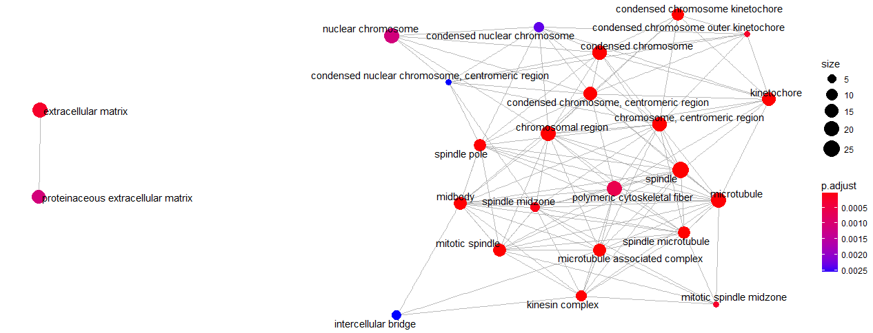
During the time of using Bioconductor packages, if any help was required you can use the following commands:
class(dnaSequence) # Indicate the class of the input object

## [1] "DNAStringSet"
## attr(,"package")
## [1] "Biostrings"

methods(class = "DNAStringSet") # List all available methods for a S3 and S4 generic function or class

##   [1] !                               !=
##   [3] $                               $<-
##   [5] %in%                            [
##   [7] [[                              [[<-
##   [9] [<-                             <
##  [11] <=                              ==
##  [13] >                               >=
##  [15] aggregate                       alphabetFrequency
##  [17] anyNA                           append
##  [19] as.character                    as.complex
##  [21] as.data.frame                   as.env
##  [23] as.factor                       as.integer
##  [25] as.list                         as.logical
##  [27] as.matrix                       as.numeric
##  [29] as.raw                          as.vector
##  [31] by                              c
##  [33] cbind                           chartr
##  [35] coerce                          compact
##  [37] compareStrings                  complement
##  [39] concatenateObjects              consensusMatrix
##  [41] consensusString                 countOverlaps
##  [43] countPattern                    countPDict
##  [45] dinucleotideFrequencyTest       do.call
##  [47] droplevels                      duplicated
##  [49] elementMetadata                 elementMetadata<-
##  [51] elementNROWS                    elementType
##  [53] eval                            expand
##  [55] expand.grid                     extractAt
##  [57] extractROWS                     Filter
##  [59] findOverlaps                    getListElement
##  [61] hasOnlyBaseLetters              head
##  [63] ifelse2                         intersect
##  [65] is.na                           is.unsorted
##  [67] isEmpty                         isMatchingEndingAt
##  [69] isMatchingStartingAt            lapply
##  [71] length                          lengths
##  [73] letterFrequency                 match
##  [75] matchPattern                    matchPDict
##  [77] mcols                           mcols<-
##  [79] merge                           metadata
##  [81] metadata<-                      mstack
##  [83] names                           names<-
##  [85] nchar                           neditEndingAt
##  [87] neditStartingAt                 NROW
##  [89] nucleotideFrequencyAt           oligonucleotideFrequency
##  [91] order                           overlapsAny
##  [93] PairwiseAlignments              PairwiseAlignmentsSingleSubject
##  [95] parallelSlotNames               parallelVectorNames
##  [97] pcompare                        pcompareRecursively
##  [99] PDict                           PWM
## [101] rank                            rbind
## [103] Reduce                          relist
## [105] relistToClass                   rename
## [107] rep                             rep.int
## [109] replaceAt                       replaceLetterAt
## [111] replaceROWS                     rev
## [113] revElements                     reverse
## [115] reverseComplement               ROWNAMES
## [117] sapply                          seqinfo
## [119] seqinfo<-                       seqlevelsInUse
## [121] seqtype                         seqtype<-
## [123] setdiff                         setequal
## [125] setListElement                  shiftApply
## [127] show                            showAsCell
## [129] sort                            split
## [131] split<-                         stack
## [133] stringDist                      strsplit
## [135] subseq                          subseq<-
## [137] subset                          subsetByOverlaps
## [139] table                           tail
## [141] tapply                          threebands
## [143] toString                        transform
## [145] translate                       trimLRPatterns
## [147] twoWayAlphabetFrequency         union
## [149] unique                          uniqueLetters
## [151] unlist                          unsplit
## [153] unstrsplit                      updateObject
## [155] values                          values<-
## [157] vcountPattern                   vcountPDict
## [159] vmatchPattern                   vwhichPDict
## [161] which.isMatchingEndingAt        which.isMatchingStartingAt
## [163] whichPDict                      width
## [165] window                          window<-
## [167] windows                         with
## [169] within                          xtabs
## [171] xvcopy                          zipdown
## see '?methods' for accessing help and source code

?complement # Show the help page of the function

## starting httpd help server ... done

browseVignettes(package="Biostrings") # Refers to all available vignettes of the input package
Furthermore, there are a lot of handy help pages and workflows available on Bioconductor sites:
By reading this tutorial, you got familiar with the Bioconductor project, and it’s fundamental role in biological research works. Besides, types of Bioconductor packages and some of the most important ones were mentioned. In the next step, a short workflow of how to install and use the project was explained. You learned how to work with Biostring and GenomicRanges packages, and as a result, you got familiar with DNA sequences and genome ranges. In another sample, you tried to apply enrichment analysis on a set of human genes. Hence, you learned the concepts of enrichment analysis and GO. In the next part, various ways of getting help during working on Bioconductor were indicated. If you would like to know more about the project, don’t hesitate to see Bioconductor_courses.
If you would like to learn more about R, take DataCamp's Experimental Design in R course.
R Courses
Course
Course
Course
blog
Summer Worsley
15 min
Tutorial
Daniel Schütte
Tutorial
Karlijn Willems
Tutorial
DataCamp Team
code-along
Ishmael Rico
code-along
Arne Warnke