群体智能算法：三个 Python 实现

粒子群优化（PSO）

粒子群优化（PSO）源于对鸟群与鱼群行为的观察。在这些自然系统中，个体根据自身的既往经验与邻居的位置移动，逐步调整以跟随群体中最成功的成员。PSO 将这一理念应用于优化问题中，让被称为粒子的智能体在搜索空间中移动，寻找最优解。

与 ACO 相比，PSO 主要在连续空间而非离散空间中运行。ACO 关注寻路与离散选择，而 PSO 更适合涉及连续变量的问题，例如参数调优。

在 PSO 中，粒子在搜索空间中探索。它们根据两个主要因素调整位置：自身已知的历史最优位置以及整个群体的全局最优位置。这种双重反馈机制使其能朝全局最优收敛。

粒子群优化的工作原理

过程从在解空间内随机初始化一群粒子开始。每个粒子代表一个可能的解。粒子移动过程中，会记住自己的个体最优位置（迄今遇到的最佳解），并被全局最优位置（任一粒子发现的最佳解）所吸引。

这种运动由“利用”和“探索”两种力量驱动：利用是在当前最佳解附近精细搜索，探索则鼓励粒子在解空间的其他区域搜索，以避免陷入局部最优。通过平衡这两种动态，PSO 能高效收敛至最佳解。

粒子群优化的 Python 实现

在金融资产组合管理中，在降低风险的同时追求最大回报的最佳资产配置并不容易。我们用 PSO 来寻找能带来最高投资回报率的资产组合。

下面的代码展示了 PSO 如何用于优化一个虚构的投资组合。它从随机的资产权重分配开始，在若干次迭代中根据有效策略不断调整，逐步找到在最低风险下实现最高回报的最优资产组合。

import numpy as np
import matplotlib.pyplot as plt

# Define the PSO parameters
class Particle:
    def __init__(self, n_assets):
        # Initialize a particle with random weights and velocities
        self.position = np.random.rand(n_assets)
        self.position /= np.sum(self.position)  # Normalize weights so they sum to 1
        self.velocity = np.random.rand(n_assets)
        self.best_position = np.copy(self.position)
        self.best_score = float('inf')  # Start with a very high score

def objective_function(weights, returns, covariance):
    """
    Calculate the portfolio's performance.
    - weights: Asset weights in the portfolio.
    - returns: Expected returns of the assets.
    - covariance: Covariance matrix representing risk.
    """
    portfolio_return = np.dot(weights, returns)  # Calculate the portfolio return
    portfolio_risk = np.sqrt(np.dot(weights.T, np.dot(covariance, weights)))  # Calculate portfolio risk (standard deviation)
    return -portfolio_return / portfolio_risk  # We want to maximize return and minimize risk

def update_particles(particles, global_best_position, returns, covariance, w, c1, c2):
    """
    Update the position and velocity of each particle.
    - particles: List of particle objects.
    - global_best_position: Best position found by all particles.
    - returns: Expected returns of the assets.
    - covariance: Covariance matrix representing risk.
    - w: Inertia weight to control particle's previous velocity effect.
    - c1: Cognitive coefficient to pull particles towards their own best position.
    - c2: Social coefficient to pull particles towards the global best position.
    """
    for particle in particles:
        # Random coefficients for velocity update
        r1, r2 = np.random.rand(len(particle.position)), np.random.rand(len(particle.position))
        # Update velocity
        particle.velocity = (w * particle.velocity +
                             c1 * r1 * (particle.best_position - particle.position) +
                             c2 * r2 * (global_best_position - particle.position))
        # Update position
        particle.position += particle.velocity
        particle.position = np.clip(particle.position, 0, 1)  # Ensure weights are between 0 and 1
        particle.position /= np.sum(particle.position)  # Normalize weights to sum to 1
        # Evaluate the new position
        score = objective_function(particle.position, returns, covariance)
        if score < particle.best_score:
            # Update the particle's best known position and score
            particle.best_position = np.copy(particle.position)
            particle.best_score = score

def pso_portfolio_optimization(n_particles, n_iterations, returns, covariance):
    """
    Perform Particle Swarm Optimization to find the optimal asset weights.
    - n_particles: Number of particles in the swarm.
    - n_iterations: Number of iterations for the optimization.
    - returns: Expected returns of the assets.
    - covariance: Covariance matrix representing risk.
    """
    # Initialize particles
    particles = [Particle(len(returns)) for _ in range(n_particles)]
    # Initialize global best position
    global_best_position = np.random.rand(len(returns))
    global_best_position /= np.sum(global_best_position)
    global_best_score = float('inf')
    
    # PSO parameters
    w = 0.5  # Inertia weight: how much particles are influenced by their own direction
    c1 = 1.5  # Cognitive coefficient: how well particles learn from their own best solutions
    c2 = 0.5  # Social coefficient: how well particles learn from global best solutions
    history = []  # To store the best score at each iteration
    
    for _ in range(n_iterations):
        update_particles(particles, global_best_position, returns, covariance, w, c1, c2)
        for particle in particles:
            score = objective_function(particle.position, returns, covariance)
            if score < global_best_score:
                # Update the global best position and score
                global_best_position = np.copy(particle.position)
                global_best_score = score
        # Store the best score (negative return/risk ratio) for plotting
        history.append(-global_best_score)
    
    return global_best_position, history

# Example data for 3 assets
returns = np.array([0.02, 0.28, 0.15])  # Expected returns for each asset
covariance = np.array([[0.1, 0.02, 0.03],  # Covariance matrix for asset risks
                       [0.02, 0.08, 0.04],
                       [0.03, 0.04, 0.07]])

# Run the PSO algorithm
n_particles = 10  # Number of particles
n_iterations = 10  # Number of iterations
best_weights, optimization_history = pso_portfolio_optimization(n_particles, n_iterations, returns, covariance)

# Plotting the optimization process
plt.figure(figsize=(12, 6))
plt.plot(optimization_history, marker='o')
plt.title('Portfolio Optimization Using PSO')
plt.xlabel('Iteration')
plt.ylabel('Objective Function Value (Negative of Return/Risk Ratio)')
plt.grid(False)  # Turn off gridlines
plt.show()

# Display the optimal asset weights
print(f"Optimal Asset Weights: {best_weights}")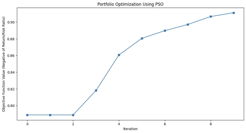技术支持

该图展示了 PSO 算法在每次迭代中对投资组合资产配置的改进程度。

粒子群优化的应用

PSO 以其简单高效而被用于解决各类优化问题，尤其是连续领域。其灵活性使其在许多需要精确解的真实场景中发挥作用。

这些应用包括：

• 机器学习：PSO 可用于机器学习算法的超参数调优，帮助找到最佳模型配置。
• 工程设计：用于优化如航天部件或电路等系统的设计参数。
• 金融建模：在金融领域用于投资组合优化，在最大化回报的同时最小化风险。

PSO 对解空间的高效探索能力使其广泛适用于从机器人到能源管理再到物流等领域。

人工蜂群（ABC）

人工蜂群（ABC）算法以蜜蜂的采蜜行为为模型。

在自然界中，蜜蜂会高效寻找花蜜源，并与蜂巢内其他成员共享信息。ABC 将这种协作搜索过程应用于优化问题，尤其适用于复杂、高维空间。

ABC 的独特之处在于它能在“利用”（精炼当前解）与“探索”（寻找新的潜在更优解）之间取得平衡。这使其在需要全局优化的大规模问题中尤为有用。

人工蜂群的工作原理

在 ABC 算法中，蜂群被分为三类角色：在职蜂、观察蜂与侦察蜂。每一角色分别模拟蜜蜂在自然中寻找与利用食源的不同方面。

• 在职蜂：负责探索已知食源，代表优化问题中的当前解。它们评估这些食源的质量（适应度），并与蜂群分享信息。
• 观察蜂：在收集在职蜂信息后，观察蜂选择哪些食源继续深挖。它们根据在职蜂分享的解的质量作出选择，更侧重更优的选项，从而精炼对最优解的搜索。
• 侦察蜂：当在职蜂的食源（解）被“榨干”或停滞（在一定次数迭代后不再改进）时，该蜂转为侦察蜂。侦察蜂探索解空间的新区域，寻找尚未开发的食源，从而为搜索过程注入多样性。

这种机制使 ABC 能在深入探索有希望的区域与广泛探索新区域之间取得平衡，帮助算法避免陷入局部最优，提高找到全局最优的概率。

人工蜂群的 Python 实现

Rastrigin 函数是优化领域的经典难题，因其存在大量局部极小值而著称，对许多算法来说颇具挑战。目标很简单：找到全局最小值。

在这个示例中，我们将使用人工蜂群算法来解决该问题。ABC 中的每只“蜜蜂”都会在搜索空间中寻找更优解以最小化该函数。代码模拟了蜜蜂的探索、利用与侦察行为，从而在探索与利用之间实现平衡。

import numpy as np
import matplotlib.pyplot as plt

# Rastrigin function: The objective is to minimize this function
def rastrigin(X):
    A = 10
    return A * len(X) + sum([(x ** 2 - A * np.cos(2 * np.pi * x)) for x in X])

# Artificial Bee Colony (ABC) algorithm for continuous optimization of Rastrigin function
def artificial_bee_colony_rastrigin(n_iter=100, n_bees=30, dim=2, bound=(-5.12, 5.12)):
    """
    Apply Artificial Bee Colony (ABC) algorithm to minimize the Rastrigin function.
    
    Parameters:
    n_iter (int): Number of iterations
    n_bees (int): Number of bees in the population
    dim (int): Number of dimensions (variables)
    bound (tuple): Bounds for the search space (min, max)
    
    Returns:
    tuple: Best solution found, best fitness value, and list of best fitness values per iteration
    """
    # Initialize the bee population with random solutions within the given bounds
    bees = np.random.uniform(bound[0], bound[1], (n_bees, dim))
    best_bee = bees[0]
    best_fitness = rastrigin(best_bee)
    
    best_fitnesses = []
    
    for iteration in range(n_iter):
        # Employed bees phase: Explore new solutions based on the current bees
        for i in range(n_bees):
            # Generate a new candidate solution by perturbing the current bee's position
            new_bee = bees[i] + np.random.uniform(-1, 1, dim)
            new_bee = np.clip(new_bee, bound[0], bound[1])  # Keep within bounds
            
            # Evaluate the fitness of the new solution
            new_fitness = rastrigin(new_bee)
            if new_fitness < rastrigin(bees[i]):
                bees[i] = new_bee  # Update bee if the new solution is better
        
        # Onlooker bees phase: Exploit good solutions
        fitnesses = np.array([rastrigin(bee) for bee in bees])
        probabilities = 1 / (1 + fitnesses)  # Higher fitness gets higher chance
        probabilities /= probabilities.sum()  # Normalize probabilities
        
        for i in range(n_bees):
            if np.random.rand() < probabilities[i]:
                selected_bee = bees[i]
                # Generate a new candidate solution by perturbing the selected bee
                new_bee = selected_bee + np.random.uniform(-0.5, 0.5, dim)
                new_bee = np.clip(new_bee, bound[0], bound[1])
                if rastrigin(new_bee) < rastrigin(selected_bee):
                    bees[i] = new_bee
        
        # Scouting phase: Randomly reinitialize some bees to explore new areas
        if np.random.rand() < 0.1:  # 10% chance to reinitialize a bee
            scout_index = np.random.randint(n_bees)
            bees[scout_index] = np.random.uniform(bound[0], bound[1], dim)
        
        # Track the best solution found so far
        current_best_bee = bees[np.argmin(fitnesses)]
        current_best_fitness = min(fitnesses)
        
        if current_best_fitness < best_fitness:
            best_fitness = current_best_fitness
            best_bee = current_best_bee
        
        best_fitnesses.append(best_fitness)
    
    return best_bee, best_fitness, best_fitnesses

# Apply ABC to minimize the Rastrigin function
best_solution, best_fitness, best_fitnesses = artificial_bee_colony_rastrigin()

# Display results
print("Best Solution (x, y):", best_solution)
print("Best Fitness (Minimum Value):", best_fitness)

# Plot the performance over iterations
plt.figure()
plt.plot(best_fitnesses)
plt.title('Performance of ABC on Rastrigin Function Optimization')
plt.xlabel('Iterations')
plt.ylabel('Best Fitness (Lower is Better)')
plt.grid(True)
plt.show()

# Plot a surface graph of the Rastrigin function
x = np.linspace(-5.12, 5.12, 200)
y = np.linspace(-5.12, 5.12, 200)
X, Y = np.meshgrid(x, y)
Z = 10 * 2 + (X ** 2 - 10 * np.cos(2 * np.pi * X)) + (Y ** 2 - 10 * np.cos(2 * np.pi * Y))

plt.figure(figsize=(8, 6))
plt.contourf(X, Y, Z, levels=50, cmap='viridis')
plt.colorbar(label='Function Value')
plt.scatter(best_solution[0], best_solution[1], c='red', label='Best Solution')
plt.title('Rastrigin Function Optimization with ABC')
plt.xlabel('X')
plt.ylabel('Y')
plt.legend()
plt.grid(True)
plt.show()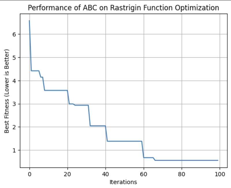技术支持

该图展示了 ABC 算法在每次迭代中找到的最佳解的适应度。在这次运行中，它大约在第 64 次迭代达到最优适应度。

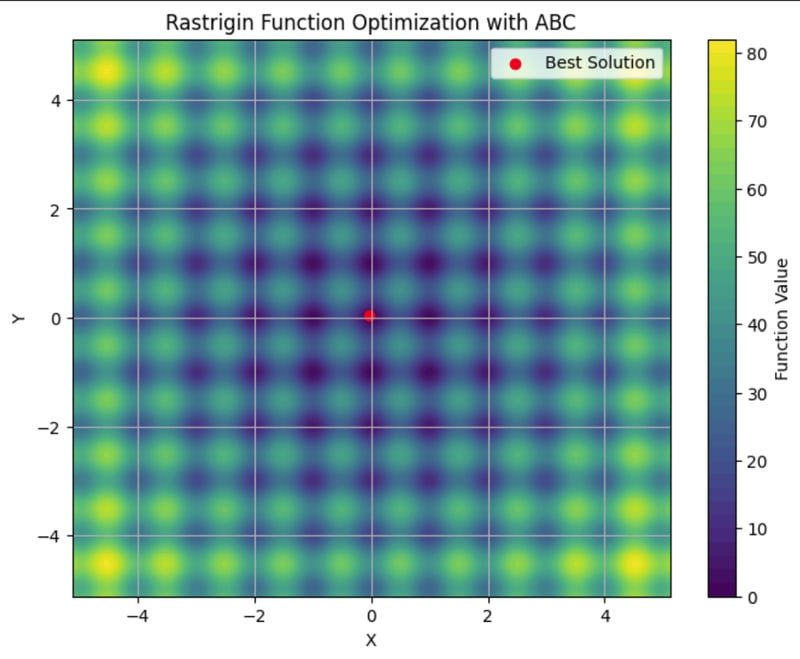
这里您可以看到 Rastrigin 函数的等高线图，包含许多局部极小值。红点是我们运行的 ABC 算法找到的全局最小值。

人工蜂群的应用

ABC 算法是解决优化问题的强健工具。其对大型、复杂搜索空间的高效探索能力，使其成为对适应性与可扩展性要求较高行业的优选方案。

这些应用包括：

• 电信通信：优化网络资源与天线的部署，在最小化成本的同时最大化覆盖与信号强度。
• 工程：用于结构设计优化中的参数微调。
• 数据科学：可用于特征选择，识别用于机器学习的最重要变量。

ABC 是一种灵活的算法，适用于需要在动态、高维环境中寻找最优解的任何问题。其去中心化特性使其在其他算法难以高效平衡探索与利用时依然表现出色。

群体智能算法对比

群体智能算法有多种，每种都有不同特性。在选择使用哪一种时，权衡其优劣以匹配您的需求非常重要。

ACO 适用于路由与调度等组合问题，但可能需要大量算力。PSO 较为简单，在连续优化（如超参数调优）方面表现出色，但可能受困于局部最优。ABC 能有效平衡探索与利用，但也需要仔细调参。

其他群体智能算法，如萤火虫算法与布谷鸟搜索优化，也为特定类型的优化问题提供独特优势。

挑战与局限

群体智能算法与许多机器学习技术一样，也会遇到影响其性能的挑战，包括：

1. 过早收敛：群体可能过快地停留在次优解上。
2. 参数调优：实现最佳结果往往需要对算法设置进行细致调整。
3. 计算资源与可扩展性：这些算法的计算开销偏大，尤其是在更大、更复杂的问题上，且随着问题复杂度提升，其性能可能下降。
4. 随机性：算法内在的随机性会导致结果存在波动。

最新研究与进展

一个显著趋势是将群体智能与其他机器学习技术相结合。研究者正在探索如何用群体算法增强特征选择与超参数优化等任务。可参阅A hybrid particle swarm optimization algorithm for solving engineering problem。

最新进展还聚焦于解决群体智能的传统挑战，如过早收敛。新的算法与技术正被开发出来，以降低收敛到次优解的风险。更多信息可查看Memory-based approaches for eliminating premature convergence in particle swarm optimization

可扩展性也是重要研究方向。随着问题愈加复杂、数据量不断增长，研究者正致力于让群体智能算法更具可扩展性与效率。这包括开发更能有效处理大数据与高维空间的算法，同时优化计算资源以降低运行这些算法的时间与成本。更多内容可参阅Recent Developments in the Theory and Applicability of Swarm Search。

群体算法正被应用于从机器人，到大语言模型（LLM），再到医疗诊断等问题领域。关于这些算法是否能帮助 LLM 为遵守Right to Be Forgotten（被遗忘权）法规而进行策略性遗忘，目前仍有持续研究。当然，群体算法在数据科学中也有诸多应用。

结论

群体智能为各行业的优化问题提供了强有力的解决方案。其去中心化、正反馈与适应等原理，使其能应对传统算法可能难以处理的复杂、动态任务。

可参考这篇关于群体算法现状的综述：“Swarm intelligence: A survey of model classification and applications”。

若想更深入了解 AI 的商业应用，请查看Artificial Intelligence (AI) Strategy 或Artificial Intelligence for Business Leaders。若想了解其他仿生算法，请查看Genetic Algorithm: Complete Guide With Python Implementation。