
Track
AI Fundamentals
10 hr
Imagine watching a flock of birds in flight. There's no leader, no one giving directions, yet they swoop and glide together in perfect harmony. It may look like chaos, but there's a hidden order. You can see the same pattern in schools of fish avoiding predators or ants finding the shortest path to food. These creatures rely on simple rules and local communication to tackle surprisingly complex tasks without central control.
That’s the magic of swarm intelligence.
We can replicate this behavior using algorithms that solve tough problems by mimicking swarm intelligence.
Swarm intelligence is a computational approach that solves complex problems by mimicking the decentralized, self-organized behavior observed in natural swarms like flocks of birds or ant colonies.
Let’s explore two key concepts: decentralization and positive feedback.
At the core of swarm intelligence is the concept of decentralization. Rather than relying on a central leader to direct actions, each individual, or "agent," operates autonomously based on limited, local information.
This decentralized decision-making leads to an emergent property—complex, organized behavior arising from the simple interactions of agents. In swarm systems, the overall outcome, or solution, is not pre-programmed but emerges naturally from these individual actions.
Take ants as an example. When foraging, an ant randomly explores its environment until it finds food, at which point it lays a pheromone trail on its way back to the colony. Other ants encounter this trail and are more likely to follow it, reinforcing the path if they find food at the end. Over time, shorter or more efficient routes naturally attract more ants as stronger pheromone trails build up along these paths. No single ant "knows" the best route from the outset, but collectively, through decentralized decisions and the reinforcement of successful paths, the colony converges on the optimal solution.
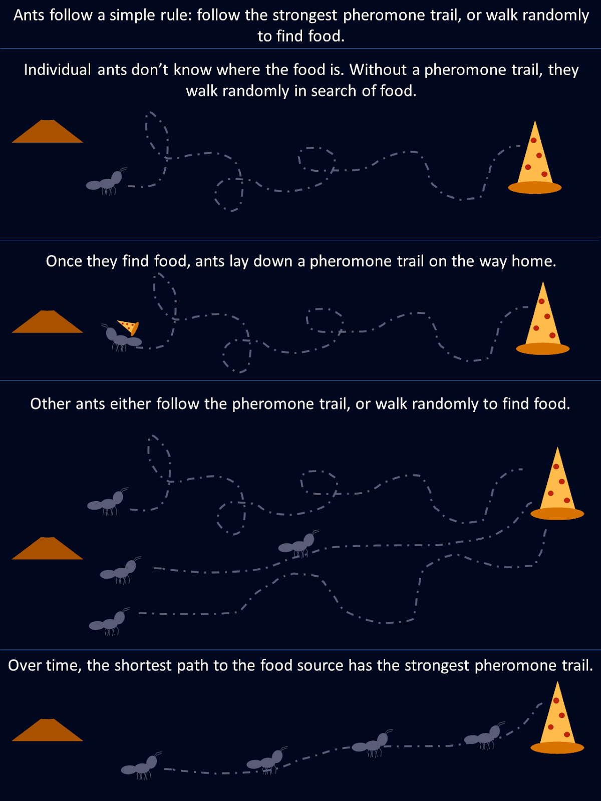
This diagram shows how simple rules followed by individual ants result in an optimal solution for the whole colony.
Positive feedback is a mechanism in swarm intelligence systems, where successful actions are rewarded and reinforced. This leads to a self-amplifying process, like the ants strengthening pheromone trails along shorter foraging paths. This reinforcement of beneficial behaviors helps the swarm improve its overall performance over time.
In artificial intelligence, swarm intelligence algorithms mimic this by adjusting key factors, such as probabilities or weights, based on the quality of the solutions found. As better solutions are discovered, agents increasingly focus on them, which accelerates the convergence process. This dynamic feedback loop allows swarm systems to adapt to changing environments and refine their performance.
There are several swarm intelligence algorithms that mimic different biological systems. Let’s go over a few of the popular ones.
Ant colony optimization (ACO) is an algorithm inspired by the foraging behavior of ants described above. It’s designed to solve combinatorial optimization problems, particularly those where we need to find the best possible solution among many. A classic example of this is the traveling salesman problem, where the goal is to determine the shortest possible route that connects a set of locations.
In nature, ants communicate by leaving behind pheromone trails, which signal to other ants the path to a food source. The more ants follow that trail, the stronger it becomes. ACO mimics this behavior with pheromones represented by mathematical values stored in a pheromone matrix. This matrix keeps track of the desirability of different solutions, and it gets updated as the algorithm progresses.
In ACO, each "artificial ant" represents a potential solution to the problem, such as a route in the traveling salesman problem. The algorithm begins with all ants randomly selecting paths, and the pheromone values help guide future ants. These values are stored in a matrix where each entry corresponds to the "pheromone level" between two points (like cities).
This mathematical representation of pheromones allows ACO to effectively balance exploration and exploitation, searching large solution spaces without getting stuck in local optima.
Let’s try an example, using ACO to solve a simple problem: find the shortest path between points on a graph.
This implementation of ACO simulates how artificial "ants" traverse 20 nodes on a graph to find the shortest path. Each ant starts at a random node and selects its next move based on pheromone trails and distances between nodes. After exploring all paths, the ants return to their starting point, completing a full loop.
Over time, pheromones are updated: the shorter paths receive stronger reinforcement, while others evaporate. This dynamic process allows the algorithm to converge toward an optimal solution.
import numpy as np
import matplotlib.pyplot as plt

# Graph class represents the environment where ants will travel
class Graph:
    def __init__(self, distances):
        # Initialize the graph with a distance matrix (distances between nodes)
        self.distances = distances
        self.num_nodes = len(distances)  # Number of nodes (cities)
        # Initialize pheromones for each path between nodes (same size as distances)
        self.pheromones = np.ones_like(distances, dtype=float)  # Start with equal pheromones

# Ant class represents an individual ant that travels across the graph
class Ant:
    def __init__(self, graph):
        self.graph = graph
        # Choose a random starting node for the ant
        self.current_node = np.random.randint(graph.num_nodes)
        self.path = [self.current_node]  # Start path with the initial node
        self.total_distance = 0  # Start with zero distance traveled
        # Unvisited nodes are all nodes except the starting one
        self.unvisited_nodes = set(range(graph.num_nodes)) - {self.current_node}

    # Select the next node for the ant to travel to, based on pheromones and distances
    def select_next_node(self):
        # Initialize an array to store the probability for each node
        probabilities = np.zeros(self.graph.num_nodes)
        # For each unvisited node, calculate the probability based on pheromones and distances
        for node in self.unvisited_nodes:
            if self.graph.distances[self.current_node][node] > 0:  # Only consider reachable nodes
                # The more pheromones and the shorter the distance, the more likely the node will be chosen
                probabilities[node] = (self.graph.pheromones[self.current_node][node] ** 2 /
                                       self.graph.distances[self.current_node][node])
        probabilities /= probabilities.sum()  # Normalize the probabilities to sum to 1
        # Choose the next node based on the calculated probabilities
        next_node = np.random.choice(range(self.graph.num_nodes), p=probabilities)
        return next_node

    # Move to the next node and update the ant's path
    def move(self):
        next_node = self.select_next_node()  # Pick the next node
        self.path.append(next_node)  # Add it to the path
        # Add the distance between the current node and the next node to the total distance
        self.total_distance += self.graph.distances[self.current_node][next_node]
        self.current_node = next_node  # Update the current node to the next node
        self.unvisited_nodes.remove(next_node)  # Mark the next node as visited

    # Complete the path by visiting all nodes and returning to the starting node
    def complete_path(self):
        while self.unvisited_nodes:  # While there are still unvisited nodes
            self.move()  # Keep moving to the next node
        # After visiting all nodes, return to the starting node to complete the cycle
        self.total_distance += self.graph.distances[self.current_node][self.path[0]]
        self.path.append(self.path[0])  # Add the starting node to the end of the path

# ACO (Ant Colony Optimization) class runs the algorithm to find the best path
class ACO:
    def __init__(self, graph, num_ants, num_iterations, decay=0.5, alpha=1.0):
        self.graph = graph
        self.num_ants = num_ants  # Number of ants in each iteration
        self.num_iterations = num_iterations  # Number of iterations
        self.decay = decay  # Rate at which pheromones evaporate
        self.alpha = alpha  # Strength of pheromone update
        self.best_distance_history = []  # Store the best distance found in each iteration

    # Main function to run the ACO algorithm
    def run(self):
        best_path = None
        best_distance = np.inf  # Start with a very large number for comparison
        # Run the algorithm for the specified number of iterations
        for _ in range(self.num_iterations):
            ants = [Ant(self.graph) for _ in range(self.num_ants)]  # Create a group of ants
            for ant in ants:
                ant.complete_path()  # Let each ant complete its path
                # If the current ant's path is shorter than the best one found so far, update the best path
                if ant.total_distance < best_distance:
                    best_path = ant.path
                    best_distance = ant.total_distance
            self.update_pheromones(ants)  # Update pheromones based on the ants' paths
            self.best_distance_history.append(best_distance)  # Save the best distance for each iteration
        return best_path, best_distance

    # Update the pheromones on the paths after all ants have completed their trips
    def update_pheromones(self, ants):
        self.graph.pheromones *= self.decay  # Reduce pheromones on all paths (evaporation)
        # For each ant, increase pheromones on the paths they took, based on how good their path was
        for ant in ants:
            for i in range(len(ant.path) - 1):
                from_node = ant.path[i]
                to_node = ant.path[i + 1]
                # Update the pheromones inversely proportional to the total distance traveled by the ant
                self.graph.pheromones[from_node][to_node] += self.alpha / ant.total_distance

# Generate random distances between nodes (cities) for a 20-node graph
num_nodes = 20
distances = np.random.randint(1, 100, size=(num_nodes, num_nodes))  # Random distances between 1 and 100
np.fill_diagonal(distances, 0)  # Distance from a node to itself is 0
graph = Graph(distances)  # Create the graph with the random distances
aco = ACO(graph, num_ants=10, num_iterations=30)  # Initialize ACO with 10 ants and 30 iterations
best_path, best_distance = aco.run()  # Run the ACO algorithm to find the best path

# Print the best path found and the total distance
print(f"Best path: {best_path}")
print(f"Total distance: {best_distance}")

# Plotting the final solution (first plot) - Shows the final path found by the ants
def plot_final_solution(distances, path):
    num_nodes = len(distances)
    # Generate random coordinates for the nodes to visualize them on a 2D plane
    coordinates = np.random.rand(num_nodes, 2) * 10
    # Plot the nodes (cities) as red points
    plt.scatter(coordinates[:, 0], coordinates[:, 1], color='red')
    # Label each node with its index number
    for i in range(num_nodes):
        plt.text(coordinates[i, 0], coordinates[i, 1], f"{i}", fontsize=10)
    # Plot the path (edges) connecting the nodes, showing the best path found
    for i in range(len(path) - 1):
        start, end = path[i], path[i + 1]
        plt.plot([coordinates[start, 0], coordinates[end, 0]],
                 [coordinates[start, 1], coordinates[end, 1]],
                 'blue', linewidth=1.5)
    plt.title("Final Solution: Best Path")
    plt.show()

# Plotting the distance over iterations (second plot) - Shows how the path length improves over time
def plot_distance_over_iterations(best_distance_history):
    # Plot the best distance found in each iteration (should decrease over time)
    plt.plot(best_distance_history, color='green', linewidth=2)
    plt.title("Trip Length Over Iterations")
    plt.xlabel("Iteration")
    plt.ylabel("Distance")
    plt.show()

# Call the plotting functions to display the results
plot_final_solution(distances, best_path)
plot_distance_over_iterations(aco.best_distance_history)![This graph shows the final solution, the best path found, to travel to each node in the shortest distance. In this run, the best route was found to be [4, 5, 17, 9, 11, 16, 13, 2, 7, 3, 6, 1, 14, 12, 18, 0, 10, 19, 15, 8, 4], with a total distance of 129.](https://media.datacamp.com/cms/google/ad_4nxcfk4zmpwq-et7v9dapocc9zbf7nm-mukhnmf83ih4ce-kh30kcuds_7ubqjmnv4ncv_iwr2nzg_oandfg1f6jc_wqkgdpu7jxlp4iilaruergyu4polxvvk5gu8x65jnuckjfj6knyoh-yqf8gpn_inper.png)
This graph shows the final solution, the best path found, to travel to each node in the shortest distance. In this run, the best route was found to be [4, 5, 17, 9, 11, 16, 13, 2, 7, 3, 6, 1, 14, 12, 18, 0, 10, 19, 15, 8, 4], with a total distance of 129.
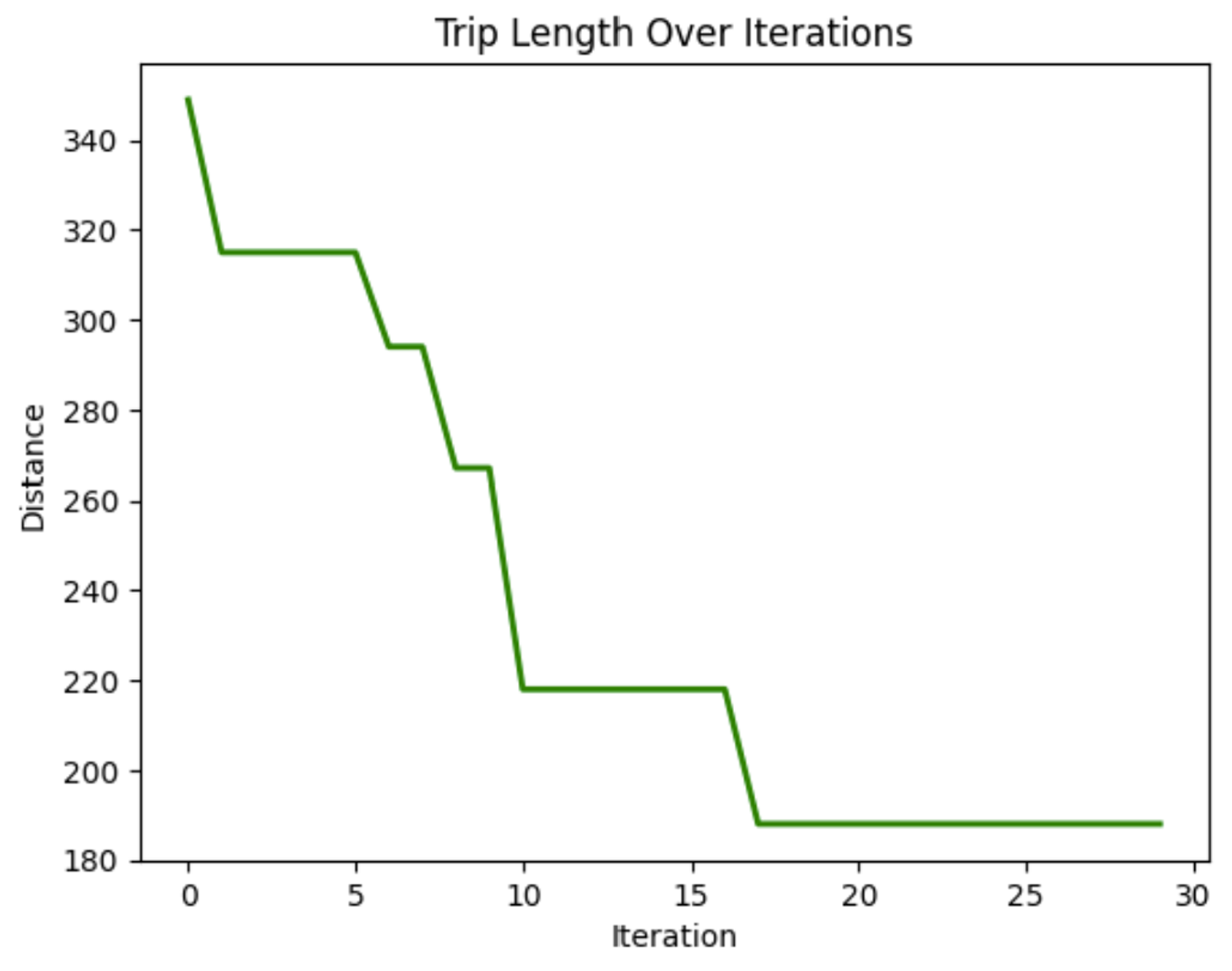
In this graph, we can see the distance traveled while traversing the nodes decreases over iterations. This demonstrates that the model is improving the trip length over time.
ACO’s adaptability and efficiency make it a powerful tool in various industries. Some applications include:
The strength of ACO lies in its ability to evolve and adapt, making it suitable for dynamic environments where conditions can change, such as real-time traffic routing or industrial planning.
Particle swarm optimization (PSO) draws its inspiration from the behavior of flocks of birds and schools of fish. In these natural systems, individuals move based on their own previous experiences and their neighbors' positions, gradually adjusting to follow the most successful members of the group. PSO applies this concept to optimization problems, where particles, called agents, move through the search space to find an optimal solution.
Compared to ACO, PSO operates in continuous rather than discrete spaces. In ACO, the focus is on pathfinding and discrete choices, while PSO is better suited for problems involving continuous variables, such as parameter tuning.
In PSO, particles explore a search space. They adjust their positions based on two main factors: their personal best-known position and the best-known position of the entire swarm. This dual feedback mechanism enables them to converge toward the global optimum.
The process starts with a swarm of particles initialized randomly across the solution space. Each particle represents a possible solution to the optimization problem. As the particles move, they remember their personal best positions (the best solution they’ve encountered so far) and are attracted toward the global best position (the best solution any particle has found).
This movement is driven by two factors: exploitation and exploration. Exploitation involves refining the search around the current best solution, while exploration encourages particles to search other parts of the solution space to avoid getting stuck in local optima. By balancing these two dynamics, PSO efficiently converges on the best solution.
In financial portfolio management, finding the best way to allocate assets to get the most returns while keeping risks low can be tricky. Let’s use a PSO to find which mix of assets will give us the highest return on investment.
The code below shows how PSO works for optimizing a fictional financial portfolio. It starts with random asset allocations, then tweaks them over several iterations based on what works best, gradually finding the optimal mix of assets for the highest return with the lowest risk.
import numpy as np
import matplotlib.pyplot as plt

# Define the PSO parameters
class Particle:
    def __init__(self, n_assets):
        # Initialize a particle with random weights and velocities
        self.position = np.random.rand(n_assets)
        self.position /= np.sum(self.position)  # Normalize weights so they sum to 1
        self.velocity = np.random.rand(n_assets)
        self.best_position = np.copy(self.position)
        self.best_score = float('inf')  # Start with a very high score

def objective_function(weights, returns, covariance):
    """
    Calculate the portfolio's performance.
    - weights: Asset weights in the portfolio.
    - returns: Expected returns of the assets.
    - covariance: Covariance matrix representing risk.
    """
    portfolio_return = np.dot(weights, returns)  # Calculate the portfolio return
    portfolio_risk = np.sqrt(np.dot(weights.T, np.dot(covariance, weights)))  # Calculate portfolio risk (standard deviation)
    return -portfolio_return / portfolio_risk  # We want to maximize return and minimize risk

def update_particles(particles, global_best_position, returns, covariance, w, c1, c2):
    """
    Update the position and velocity of each particle.
    - particles: List of particle objects.
    - global_best_position: Best position found by all particles.
    - returns: Expected returns of the assets.
    - covariance: Covariance matrix representing risk.
    - w: Inertia weight to control particle's previous velocity effect.
    - c1: Cognitive coefficient to pull particles towards their own best position.
    - c2: Social coefficient to pull particles towards the global best position.
    """
    for particle in particles:
        # Random coefficients for velocity update
        r1, r2 = np.random.rand(len(particle.position)), np.random.rand(len(particle.position))
        # Update velocity
        particle.velocity = (w * particle.velocity +
                             c1 * r1 * (particle.best_position - particle.position) +
                             c2 * r2 * (global_best_position - particle.position))
        # Update position
        particle.position += particle.velocity
        particle.position = np.clip(particle.position, 0, 1)  # Ensure weights are between 0 and 1
        particle.position /= np.sum(particle.position)  # Normalize weights to sum to 1
        # Evaluate the new position
        score = objective_function(particle.position, returns, covariance)
        if score < particle.best_score:
            # Update the particle's best known position and score
            particle.best_position = np.copy(particle.position)
            particle.best_score = score

def pso_portfolio_optimization(n_particles, n_iterations, returns, covariance):
    """
    Perform Particle Swarm Optimization to find the optimal asset weights.
    - n_particles: Number of particles in the swarm.
    - n_iterations: Number of iterations for the optimization.
    - returns: Expected returns of the assets.
    - covariance: Covariance matrix representing risk.
    """
    # Initialize particles
    particles = [Particle(len(returns)) for _ in range(n_particles)]
    # Initialize global best position
    global_best_position = np.random.rand(len(returns))
    global_best_position /= np.sum(global_best_position)
    global_best_score = float('inf')

    # PSO parameters
    w = 0.5  # Inertia weight: how much particles are influenced by their own direction
    c1 = 1.5  # Cognitive coefficient: how well particles learn from their own best solutions
    c2 = 0.5  # Social coefficient: how well particles learn from global best solutions
    history = []  # To store the best score at each iteration

    for _ in range(n_iterations):
        update_particles(particles, global_best_position, returns, covariance, w, c1, c2)
        for particle in particles:
            score = objective_function(particle.position, returns, covariance)
            if score < global_best_score:
                # Update the global best position and score
                global_best_position = np.copy(particle.position)
                global_best_score = score
        # Store the best score (negative return/risk ratio) for plotting
        history.append(-global_best_score)

    return global_best_position, history

# Example data for 3 assets
returns = np.array([0.02, 0.28, 0.15])  # Expected returns for each asset
covariance = np.array([[0.1, 0.02, 0.03],  # Covariance matrix for asset risks
                       [0.02, 0.08, 0.04],
                       [0.03, 0.04, 0.07]])

# Run the PSO algorithm
n_particles = 10  # Number of particles
n_iterations = 10  # Number of iterations
best_weights, optimization_history = pso_portfolio_optimization(n_particles, n_iterations, returns, covariance)

# Plotting the optimization process
plt.figure(figsize=(12, 6))
plt.plot(optimization_history, marker='o')
plt.title('Portfolio Optimization Using PSO')
plt.xlabel('Iteration')
plt.ylabel('Objective Function Value (Negative of Return/Risk Ratio)')
plt.grid(False)  # Turn off gridlines
plt.show()

# Display the optimal asset weights
print(f"Optimal Asset Weights: {best_weights}")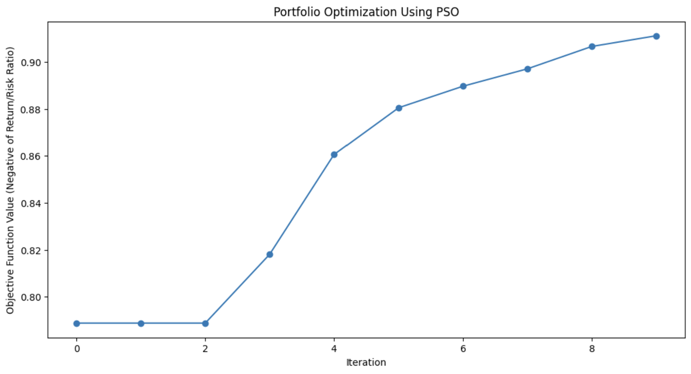
This graph demonstrates how much the PSO algorithm improved the portfolio’s asset mix with each iteration.
PSO is used for its simplicity and effectiveness in solving various optimization problems, particularly in continuous domains. Its flexibility makes it useful for many real-world scenarios where precise solutions are needed.
These applications include:
PSO's ability to efficiently explore solution spaces makes it applicable across fields, from robotics to energy management to logistics.
The artificial bee colony (ABC) algorithm is modeled on the foraging behavior of honeybees.
In nature, honeybees efficiently search for nectar sources and share this information with other members of the hive. ABC captures this collaborative search process and applies it to optimization problems, especially those involving complex, high-dimensional spaces.
What sets ABC apart from other swarm intelligence algorithms is its ability to balance exploitation, focusing on refining current solutions, and exploration, searching for new and potentially better solutions. This makes ABC particularly useful for large-scale problems where global optimization is key.
In the ABC algorithm, the swarm of bees is divided into three specialized roles: employed bees, onlookers, and scouts. Each of these roles mimics a different aspect of how bees search for and exploit food sources in nature.
This dynamic allows ABC to balance the search between intensively exploring promising areas and broadly exploring new areas of the search space. This helps the algorithm avoid getting trapped in local optima and increases its chances of finding a global optimum.
The Rastrigin function is a popular problem in optimization, known for its numerous local minima, making it a tough challenge for many algorithms. The goal is simple: find the global minimum.
In this example, we’ll use the artificial bee colony algorithm to tackle this problem. Each bee in the ABC algorithm explores the search space, looking for better solutions to minimize the function. The code simulates bees that explore, exploit, and scout for new areas, ensuring a balance between exploration and exploitation.
import numpy as np
import matplotlib.pyplot as plt

# Rastrigin function: The objective is to minimize this function
def rastrigin(X):
    A = 10
    return A * len(X) + sum([(x ** 2 - A * np.cos(2 * np.pi * x)) for x in X])

# Artificial Bee Colony (ABC) algorithm for continuous optimization of Rastrigin function
def artificial_bee_colony_rastrigin(n_iter=100, n_bees=30, dim=2, bound=(-5.12, 5.12)):
    """
    Apply Artificial Bee Colony (ABC) algorithm to minimize the Rastrigin function.

    Parameters:
    n_iter (int): Number of iterations
    n_bees (int): Number of bees in the population
    dim (int): Number of dimensions (variables)
    bound (tuple): Bounds for the search space (min, max)

    Returns:
    tuple: Best solution found, best fitness value, and list of best fitness values per iteration
    """
    # Initialize the bee population with random solutions within the given bounds
    bees = np.random.uniform(bound[0], bound[1], (n_bees, dim))
    best_bee = bees[0]
    best_fitness = rastrigin(best_bee)

    best_fitnesses = []

    for iteration in range(n_iter):
        # Employed bees phase: Explore new solutions based on the current bees
        for i in range(n_bees):
            # Generate a new candidate solution by perturbing the current bee's position
            new_bee = bees[i] + np.random.uniform(-1, 1, dim)
            new_bee = np.clip(new_bee, bound[0], bound[1])  # Keep within bounds

            # Evaluate the fitness of the new solution
            new_fitness = rastrigin(new_bee)
            if new_fitness < rastrigin(bees[i]):
                bees[i] = new_bee  # Update bee if the new solution is better

        # Onlooker bees phase: Exploit good solutions
        fitnesses = np.array([rastrigin(bee) for bee in bees])
        probabilities = 1 / (1 + fitnesses)  # Higher fitness gets higher chance
        probabilities /= probabilities.sum()  # Normalize probabilities

        for i in range(n_bees):
            if np.random.rand() < probabilities[i]:
                selected_bee = bees[i]
                # Generate a new candidate solution by perturbing the selected bee
                new_bee = selected_bee + np.random.uniform(-0.5, 0.5, dim)
                new_bee = np.clip(new_bee, bound[0], bound[1])
                if rastrigin(new_bee) < rastrigin(selected_bee):
                    bees[i] = new_bee

        # Scouting phase: Randomly reinitialize some bees to explore new areas
        if np.random.rand() < 0.1:  # 10% chance to reinitialize a bee
            scout_index = np.random.randint(n_bees)
            bees[scout_index] = np.random.uniform(bound[0], bound[1], dim)

        # Track the best solution found so far
        current_best_bee = bees[np.argmin(fitnesses)]
        current_best_fitness = min(fitnesses)

        if current_best_fitness < best_fitness:
            best_fitness = current_best_fitness
            best_bee = current_best_bee

        best_fitnesses.append(best_fitness)

    return best_bee, best_fitness, best_fitnesses

# Apply ABC to minimize the Rastrigin function
best_solution, best_fitness, best_fitnesses = artificial_bee_colony_rastrigin()

# Display results
print("Best Solution (x, y):", best_solution)
print("Best Fitness (Minimum Value):", best_fitness)

# Plot the performance over iterations
plt.figure()
plt.plot(best_fitnesses)
plt.title('Performance of ABC on Rastrigin Function Optimization')
plt.xlabel('Iterations')
plt.ylabel('Best Fitness (Lower is Better)')
plt.grid(True)
plt.show()

# Plot a surface graph of the Rastrigin function
x = np.linspace(-5.12, 5.12, 200)
y = np.linspace(-5.12, 5.12, 200)
X, Y = np.meshgrid(x, y)
Z = 10 * 2 + (X ** 2 - 10 * np.cos(2 * np.pi * X)) + (Y ** 2 - 10 * np.cos(2 * np.pi * Y))

plt.figure(figsize=(8, 6))
plt.contourf(X, Y, Z, levels=50, cmap='viridis')
plt.colorbar(label='Function Value')
plt.scatter(best_solution[0], best_solution[1], c='red', label='Best Solution')
plt.title('Rastrigin Function Optimization with ABC')
plt.xlabel('X')
plt.ylabel('Y')
plt.legend()
plt.grid(True)
plt.show()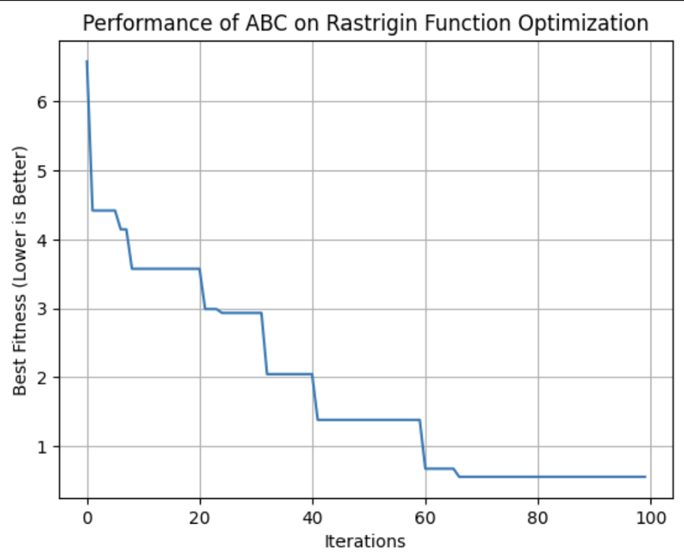
This graph shows the fitness of the best solution found by the ABC algorithm with each iteration. In this run, it reached its optimum fitness around the 64th iteration.
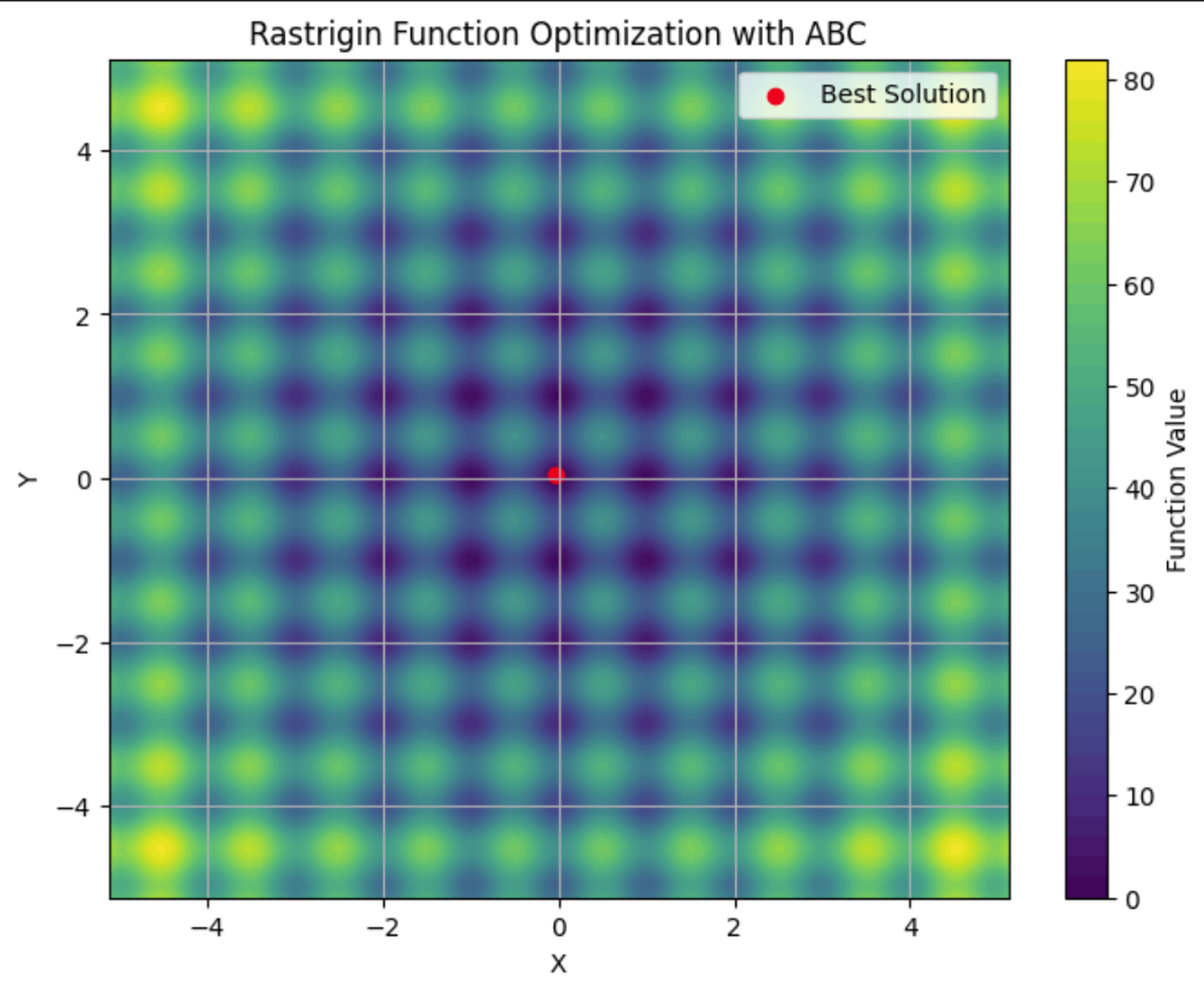
Here you can see the Rastrigin function plotted on a contour plot, with its many local minima. The red dot is the global minima found by the ABC algorithm we ran.
The ABC algorithm is a robust tool for solving optimization problems. Its ability to efficiently explore large and complex search spaces makes it a go-to choice for industries where adaptability and scalability are critical.
These applications include:
ABC is a flexible algorithm suitable for any problem where optimal solutions need to be found in dynamic, high-dimensional environments. Its decentralized nature makes it well-suited for situations where other algorithms may struggle to balance exploration and exploitation efficiently.
There are multiple swarm intelligence algorithms, each with different attributes. When deciding which to use, it's important to weigh their strengths and weaknesses to decide which best suits your needs.
ACO is effective for combinatorial problems like routing and scheduling but may need significant computational resources. PSO is simpler and excels in continuous optimization, such as hyperparameter tuning, but can struggle with local optima. ABC successfully balances exploration and exploitation, though it requires careful tuning.
Other swarm intelligence algorithms, such as Firefly Algorithm and Cuckoo Search Optimization, also offer unique advantages for specific types of optimization problems.
|
Algorithm |
Strengths |
Weaknesses |
Preferred Libraries |
Best Applications |
|
Ant Colony Optimization (ACO) |
Effective for combinatorial problems and handles complex discrete spaces well |
Computationally intensive and requires fine-tuning |
Routing problems, scheduling, and resource allocation |
|
|
Particle Swarm Optimization (PSO) |
Good for continuous optimization and simple and easy to implement |
Can converge to local optima and is less effective for discrete problems |
Hyperparameter tuning, engineering design, financial modeling |
|
|
Artificial Bee Colony (ABC) |
Adaptable to large, dynamic problems and balanced exploration and exploitation |
Computationally intensive and requires careful parameter tuning |
Telecommunications, large-scale optimization, and high-dimensional spaces |
|
|
Firefly Algorithm (FA) |
Excels in multimodal optimization and has strong global search ability |
Sensitive to parameter settings and slower convergence |
Image processing, engineering design, and multimodal optimization |
|
|
Cuckoo Search (CS) |
Efficient for solving optimization problems and has strong exploration capabilities |
May converge prematurely and performance depends on tuning |
Scheduling, feature selection, and engineering applications |
Swarm intelligence algorithms, like many machine learning techniques, encounter challenges that can affect their performance. These include:
A notable trend is the integration of swarm intelligence with other machine learning techniques. Researchers are exploring how swarm algorithms can enhance tasks such as feature selection and hyperparameter optimization. Check out A hybrid particle swarm optimization algorithm for solving engineering problem.
Recent advancements also focus on addressing some of the traditional challenges associated with swarm intelligence, such as premature convergence. New algorithms and techniques are being developed to mitigate the risk of converging on suboptimal solutions. For more information, check out Memory-based approaches for eliminating premature convergence in particle swarm optimization
Scalability is another significant area of research. As problems become increasingly complex and data volumes grow, researchers are working on ways to make swarm intelligence algorithms more scalable and efficient. This includes developing algorithms that can handle large datasets and high-dimensional spaces more effectively, while optimizing computational resources to reduce the time and cost associated with running these algorithms. For more on this, check out Recent Developments in the Theory and Applicability of Swarm Search.
Swarm algorithms are being applied to problems from robotics, to large language models (LLMs), to medical diagnosis. There is ongoing research into whether these algorithms can be useful for helping LLMs strategically forget information to comply with Right to Be Forgotten regulations. And, of course, swarm algorithms have a multitude of applications in data science.
Swarm intelligence offers powerful solutions for optimization problems across various industries. Its principles of decentralization, positive feedback, and adaptation allow it to tackle complex, dynamic tasks that traditional algorithms might struggle with.
Check out this review of the current state of swarm algorithms, “Swarm intelligence: A survey of model classification and applications”.
For a deeper dive into the business applications of AI, check out Artificial Intelligence (AI) Strategy or Artificial Intelligence for Business Leaders. To learn about other algorithms that imitate nature, check out Genetic Algorithm: Complete Guide With Python Implementation.
Learn AI with these courses!
Track
Course
Course
Tutorial
Rajesh Kumar
Tutorial
Amberle McKee
Tutorial
Bex Tuychiev
Tutorial
Arun Nanda
Tutorial
Amberle McKee
Tutorial
Bex Tuychiev