Data Science in Banking: Fraud Detection

• Data Science Use Case in Banking: Detecting Fraud 
• Preparing the Dataset
• Calculating Fraud in the Dataset
• Using SMOTE to Re-Balance the Data
• Applying Logistic Regression 
• Conclusion

Banking is one of those lucky fields where historically a lot of structured data is collected, and also one of the first where data science technologies were applied.

How is data science used in banking? Nowadays, data has become the most valuable asset in this sphere. Data science is a necessary requirement for banks to keep up with their rivals, attract more clients, increase the loyalty of existing clients, make more efficient data-driven decisions, empower their business, enhance operational efficiency, improve existing services/products and introduce new ones, reinforce security, and, as a result of all these actions, obtain more revenue. It is not surprising that the majority of all data science job demand comes from banking.

Data science allows the banking industry to successfully perform numerous tasks, including: 

• investment risk analysis
• customer lifetime value prediction
• customer segmentation
• customer churn rate prediction
• personalized marketing
• customer sentiment analysis
• virtual assistants and chatbots

Below, we'll take a closer look at one of the most common data science use cases in banking.

Data Science Use Case in Banking: Detecting Fraud 

Fraudulent activities represent a challenging problem not only in banking but also in many other spheres, such as government, insurance, public sector, sales, and healthcare. Any business that deals with a high number of online transactions runs a significant risk of fraud. Financial crimes can take various forms, including fraudulent credit card transactions, forged bank checks, tax evasion, money laundering, cyber attacks, customer account theft, synthetic identities, fake applications, and scams.

Fraud detection is a set of proactive measures undertaken to identify and prevent fraudulent activities and financial losses. Its main analytical techniques can be divided into two groups:

• Statistical: statistical parameter calculation, regression, probability distributions, data matching
• Artificial intelligence (AI): data mining, machine learning, deep learning

Machine learning represents an essential pillar for fraud detection. Its toolkit provides two approaches:

• Supervised methods: k-nearest neighbors, logistic regression, support vector machines, decision tree, random forest, time-series analysis, neural networks, etc.
• Unsupervised methods: cluster analysis, link analysis, self-organizing maps, principal component analysis, anomaly recognition, etc.

There is no universal and reliable machine learning algorithm for fraud detection. Instead, for the real-world data science use cases, several techniques or their combinations are usually tested, the model predictive accuracy is calculated, and the optimal approach is selected.

The main challenge for fraud detection systems is to rapidly adapt to constantly changing fraud patterns and fraudsters' tactics and to promptly uncover new and increasingly elaborate schemes. Fraud cases are always in a minority and are well concealed among the real transactions.

Preparing the Dataset

Let's explore a machine learning implementation of credit card fraud detection using Python programming language. We'll work on the creditcard_data dataset, which is a modified sample from a Kaggle dataset on Credit Card Fraud Detection. The original data represents transactions made on credit cards owned by European cardholders in two days in September 2013.

Let's import the data and take a quick look at it:

import pandas as pd

creditcard_data = pd.read_csv('creditcard_data.csv', index_col=0)
print(creditcard_data.info())
print('\n')
pd.options.display.max_columns = len(creditcard_data)
print(creditcard_data.head(3))Powered by

<class 'pandas.core.frame.DataFrame'>
Int64Index: 5050 entries, 0 to 5049
Data columns (total 30 columns):
#   Column  Non-Null Count  Dtype 
---  ------  --------------  ----- 
0   V1      5050 non-null   float64
1   V2      5050 non-null   float64
2   V3      5050 non-null   float64
3   V4      5050 non-null   float64
4   V5      5050 non-null   float64
5   V6      5050 non-null   float64
6   V7      5050 non-null   float64
7   V8      5050 non-null   float64
8   V9      5050 non-null   float64
9   V10     5050 non-null   float64
10  V11     5050 non-null   float64
11  V12     5050 non-null   float64
12  V13     5050 non-null   float64
13  V14     5050 non-null   float64
14  V15     5050 non-null   float64
15  V16     5050 non-null   float64
16  V17     5050 non-null   float64
17  V18     5050 non-null   float64
18  V19     5050 non-null   float64
19  V20     5050 non-null   float64
20  V21     5050 non-null   float64
21  V22     5050 non-null   float64
22  V23     5050 non-null   float64
23  V24     5050 non-null   float64
24  V25     5050 non-null   float64
25  V26     5050 non-null   float64
26  V27     5050 non-null   float64
27  V28     5050 non-null   float64
28  Amount  5050 non-null   float64
29  Class   5050 non-null   int64 
dtypes: float64(29), int64(1)
memory usage: 1.2 MB


        V1        V2        V3        V4        V5        V6        V7  \
0  1.725265 -1.337256 -1.012687 -0.361656 -1.431611 -1.098681 -0.842274  
1  0.683254 -1.681875  0.533349 -0.326064 -1.455603  0.101832 -0.520590  
2  1.067973 -0.656667  1.029738  0.253899 -1.172715  0.073232 -0.745771  

        V8        V9       V10       V11       V12       V13       V14  \
0 -0.026594 -0.032409  0.215113  1.618952 -0.654046 -1.442665 -1.546538  
1  0.114036 -0.601760  0.444011  1.521570  0.499202 -0.127849 -0.237253  
2  0.249803  1.383057 -0.483771 -0.782780  0.005242 -1.273288 -0.269260  

        V15       V16       V17       V18       V19       V20       V21  \
0 -0.230008  1.785539  1.419793  0.071666  0.233031  0.275911  0.414524  
1 -0.752351  0.667190  0.724785 -1.736615  0.702088  0.638186  0.116898  
2  0.091287 -0.347973  0.495328 -0.925949  0.099138 -0.083859 -0.189315  

        V22       V23       V24       V25       V26       V27       V28  \
0  0.793434  0.028887  0.419421 -0.367529 -0.155634 -0.015768  0.010790  
1 -0.304605 -0.125547  0.244848  0.069163 -0.460712 -0.017068  0.063542  
2 -0.426743  0.079539  0.129692  0.002778  0.970498 -0.035056  0.017313  

  Amount  Class 
0  189.00      0 
1  315.17      0 
2   59.98      0 Powered by

The dataset contains the following variables:

• Numerically encoded variables V1 to V28 which are the principal components obtained from a PCA transformation. Due to confidentiality issues, no background information about the original features was provided.
• The Amount variable represents the transaction amount.
• The Class variable shows whether the transaction was a fraud (1) or not (0).

By their nature, fraud occurrences are fortunately an extreme minority in any list of transactions. However, machine learning algorithms usually work best when the different classes contained in the dataset are more or less equally present.  Otherwise, there's little data to learn from. This problem is called the class imbalance.

Calculating Fraud in the Dataset

Let's calculate the percentage of fraudulent transactions over the total number of transactions in our dataset:

round(creditcard_data['Class'].value_counts()*100/len(creditcard_data)).convert_dtypes()Powered by

0    99
1     1
Name: Class, dtype: Int64Powered by

and create a plot to visualize the fraud to non-fraud data points:

import matplotlib.pyplot as plt
import numpy as np

def prep_data(df):
    X = df.iloc[:, 1:28]
    X = np.array(X).astype(float)
    y = df.iloc[:, 29]
    y = np.array(y).astype(float)
    return X, y

def plot_data(X, y):
    plt.scatter(X[y==0, 0], X[y==0, 1], label='Class #0', alpha=0.5, linewidth=0.15)
    plt.scatter(X[y==1, 0], X[y==1, 1], label='Class #1', alpha=0.5, linewidth=0.15, c='r')
    plt.legend()
    return plt.show()

X, y = prep_data(creditcard_data)

plot_data(X, y)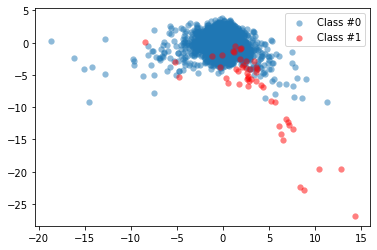Powered by

Using SMOTE to Re-Balance the Data 

We can confirm now that the ratio of fraudulent transactions is very low and that we have a case of the class imbalance problem. To fix it, we can re-balance our data using the synthetic minority oversampling technique (SMOTE). Unlike random oversampling, SMOTE is slightly more sophisticated since it doesn't just create exact copies of observations. Instead, it uses characteristics of nearest neighbors of fraud cases to create new, synthetic samples that are quite similar to the existing observations in the minority class. Let's apply SMOTE to our credit card data:

from imblearn.over_sampling import SMOTE

method = SMOTE()
X_resampled, y_resampled = method.fit_resample(X, y)
plot_data(X_resampled, y_resampled)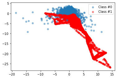Powered by

As we can see, using SMOTE suddenly gives us more observations of the minority class. To see the results of this approach even better, we'll compare them to the original data:

def compare_plot(X, y, X_resampled, y_resampled, method):
    f, (ax1, ax2) = plt.subplots(1, 2)
    c0 = ax1.scatter(X[y==0, 0], X[y==0, 1], label='Class #0',alpha=0.5)
    c1 = ax1.scatter(X[y==1, 0], X[y==1, 1], label='Class #1',alpha=0.5, c='r')
    ax1.set_title('Original set')
    ax2.scatter(X_resampled[y_resampled==0, 0], X_resampled[y_resampled==0, 1], label='Class #0', alpha=.5)
    ax2.scatter(X_resampled[y_resampled==1, 0], X_resampled[y_resampled==1, 1], label='Class #1', alpha=.5,c='r')
    ax2.set_title(method)
    plt.figlegend((c0, c1), ('Class #0', 'Class #1'), loc='lower center', ncol=2, labelspacing=0.)
    plt.tight_layout(pad=3)
    return plt.show()

print(f'Original set:\n'
      f'{pd.value_counts(pd.Series(y))}\n\n'
      f'SMOTE:\n'
      f'{pd.value_counts(pd.Series(y_resampled))}\n')

compare_plot(X, y, X_resampled, y_resampled, method='SMOTE')Powered by

Original set:
0.0    5000
1.0      50
dtype: int64


SMOTE:
0.0    5000
1.0    5000
dtype: int64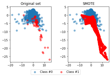Powered by

Hence, the SMOTE method has balanced our data completely, and the minority class is now equal in size to the majority class.

We'll return to the practical application of the SMOTE method soon, but for now, let's come back to the original data and try to detect the fraud cases. Following the "old-school" way, we have to create some rules to catch fraud. Such rules can concern, for example, unusual locations of transactions or suspiciously frequent transactions. The idea is to define threshold values based on common statistics, often on the mean values of observations, and use those thresholds on our features to detect fraud.

print(creditcard_data.groupby('Class').mean().round(3)[['V1', 'V3']])Powered by

        V1     V3
Class             
0      0.035  0.037
1     -4.985 -7.294Powered by

In our particular case, let's apply the following conditions: V1 < -3 and V3 < -5. Then, to estimate the performance of this approach, we'll compare the flagged fraud cases to the actual ones:

creditcard_data['flag_as_fraud'] = np.where(np.logical_and(creditcard_data['V1']<-3, creditcard_data['V3']<-5), 1, 0)
print(pd.crosstab(creditcard_data['Class'], creditcard_data['flag_as_fraud'], rownames=['Actual Fraud'], colnames=['Flagged Fraud']))Powered by

Flagged Fraud     0   1
Actual Fraud          
0              4984  16
1                28  22Powered by

Applying Logistic Regression 

We detected 22 out of 50 fraud cases, but can't detect the other 28, and got 16 false positives. Let's see if using machine learning techniques can beat those results.

We're now going to implement a simple logistic regression classification algorithm on our credit card data to identify fraudulent occurrences and then visualize the results on a confusion matrix:

from sklearn.model_selection import train_test_split
from sklearn.linear_model import LogisticRegression

X_train, X_test, y_train, y_test = train_test_split(X, y, test_size=0.3, random_state=0)

lr = LogisticRegression()
lr.fit(X_train, y_train)
predictions = lr.predict(X_test)
print(pd.crosstab(y_test, predictions, rownames=['Actual Fraud'], colnames=['Flagged Fraud']))Powered by

Flagged Fraud   0.0  1.0
Actual Fraud           
0.0            1504    1
1.0             1      9Powered by

It's important to note that here we have fewer observations to look at in the confusion matrix because we're only using the test set to calculate the model results on, i.e., only 30% of the whole dataset.

We caught a higher percentage of fraud cases: 90% (9 out of 10), compared to the previous result of 44% (22 out of 50). We also got far fewer false positives than before, so that's an improvement.

Let's now return to the class imbalance problem discussed earlier and explore whether we can enhance the prediction results even further by combining the logistic regression model with the SMOTE resampling method. To do it efficiently and in one go, we need to define a pipeline and run it on our data:

from imblearn.pipeline import Pipeline

# Defining which resampling method and which ML model to use in the pipeline
resampling = SMOTE()
lr = LogisticRegression()

pipeline = Pipeline([('SMOTE', resampling), ('Logistic Regression', lr)])
pipeline.fit(X_train, y_train)
predictions = pipeline.predict(X_test)
print(pd.crosstab(y_test, predictions, rownames=['Actual Fraud'], colnames=['Flagged Fraud']))Powered by

Flagged Fraud   0.0  1.0
Actual Fraud           
0.0            1496    9
1.0               1    9Powered by

As we can see, in our case the SMOTE didn't bring any improvements: we still caught 90% of fraud occurrences and, moreover, we have a slightly higher number of false positives. The explanation here is that resampling doesn’t necessarily lead to better results in all cases. When the fraud cases are very spread out over the data, their nearest neighbors aren't necessarily also fraud cases, so using SMOTE can introduce a bias.

Conclusion 

As a possible way forward, to increase the logistic regression model accuracy, we can tune some of the algorithm parameters. K-fold cross-validation can also be considered instead of just splitting the dataset into two parts. Finally, we can try some other machine learning algorithms (e.g., decision tree or random forest) and see if they give better results. 

If you want to learn more about the theoretical and technical aspects of fraud detection model implementation, you can explore the materials of the Fraud Detection in Python course.