Data Science: Definition and Practical Applications
Data science is a relatively recent yet fast-growing and multifaceted field of study used in many spheres. It uses various advanced analytics techniques and predictive modeling algorithms to extract meaningful insights from data to help answer strategic business or scientific questions. Data science combines a wide range of skills, from technical (programming, linear algebra, statistics, and modeling) to non-technical ones (efficient representation and communication of the results). In addition, depending on the industry where data science is applied, it's necessary to have solid domain knowledge to be able to correctly interpret the available information and the obtained insights.
Data science algorithms can be successfully applied to diverse settings where a lot of data is or can be collected: finance, commerce, marketing, project management, insurance, medicine, education, manufacturing, HR, linguistics, sociology, etc. Practically, any industry or science can benefit significantly from gathering, collecting, analyzing, and modeling their data.
What is a Data Science Use Case?
A data science use case is a concrete real-world task to be solved using the available data. In the framework of a particular company, many variables are analyzed using data science techniques in the context of the company’s specific industry. Data science use cases can be a problem to be resolved, a hypothesis to be checked, or a question to be answered. Essentially, doing data science means solving real-world use cases.
Although the content of each use case will likely be very different, there are some common things to always keep in mind:
- Data science use case planning is: outlining a clear goal and expected outcomes, understanding the scope of work, assessing available resources, providing required data, evaluating risks, and defining KPI as a measure of success.
- The most common approaches to solving data science use cases are: forecasting, classification, pattern and anomaly detection, recommendations, and image recognition.
- Some data science use cases represent typical tasks across different fields and you can rely on similar approaches to solve them, such as customer churn rate prediction, customer segmentation, fraud detection, recommendation systems, and price optimization.
How Do I Solve a Data Science Case Study?
The answer to this question is very case-specific, driven by the company's business strategy, and depending on the core of the case study itself. However, it can be helpful to outline a general roadmap to follow with any data science use case:
- Formulating the right question. This first step is very important and includes reviewing available literature and existing case studies, revising best practices, elaborating relevant theories and working hypotheses, and filling up potential gaps in domain expertise. As a result, we should come up with a clear question to be answered in the case study of interest.
- Data collection. At this step, we conduct a data inventory and gathering process. In real life, we often have non-representative, incomplete, flawed, and unstructured data, i.e. far away from being a complete table of information that is easy to read and ready to be analyzed. Therefore, we have to search for and identify all possible data sources that could be useful for our topic. The necessary data can be found in the company's archives, web-scraped, or acquired from a sponsor, etc.
- Data wrangling. This is usually the most time- and resource-consuming part of any data science project. The quality and representativeness of the gathered data are estimated and initial data exploration is conducted. The data is cleaned, preprocessed, transformed, manipulated, and mapped from its raw form into a more suitable format.
- Data analysis and modeling. The cleaned data is analyzed from the standpoint of its current status, then fit into a selected predictive statistical model. The model accuracy is evaluated and, if not satisfactory, other modeling approaches are tried. This is repeated until the model that predicts future scenarios with the highest precision has been obtained. Hence this process, as all the previous ones, can be quite iterative.
- Result communication. In comparison to the previous steps, this one requires more communication and soft skills rather than programming and technical expertise. It includes sharing the most important findings and ultimate conclusions with management, shareholders, and any other involved parties. The insights are commonly represented in the form of reports, articles, and presentation slides, outlining potential ways forward.
Data Science Use Cases by Industry
Data science use cases can be related to virtually any industry where a large amount of data is or can be accumulated. In this chapter, we're going to discuss some typical data science use cases from the following most in-demand fields: logistics, healthcare, and telecommunications. Some of the use cases that we're going to consider are interdisciplinary and can be easily encountered in many other spheres. This makes them more universal and applicable, so it's worth knowing an overall approach to solving them. In addition, for each of the selected industries, we'll outline some other possible topics that can be modeled with data science methods.
Data Science in Healthcare
In the previous three chapters, we have discussed how data science methods can help companies from different industries to increase their revenue. When it comes to healthcare, not only can the correct usage and interpretation of available data be beneficial for the marketeers of this sector, but it can also help the timely diagnosis of serious diseases and even save people's lives.
Medicine and healthcare providers gather a huge amount of data from numerous sources: electronic health record (EHR) systems, data from wearable devices, medical research studies, and billing documents. Taking advantage of innovative data science and data analysis techniques is gradually revolutionizing the whole industry of healthcare, offering the most promising and impactful solutions for its future development. In particular, some highly specialized fields of healthcare such as genetics, reproductive medicine, oncology, biotechnology, radiography, predictive diagnostics, and pharmaceutics have moved to a completely new level thanks to unlocking the full potential of their data.
To get a better understanding of how data science can be of value in medicine, let's focus on one of the most classic use cases.
Data science use case in healthcare: Breast cancer prediction
According to the World Cancer Research Fund International, breast cancer is the most common cancer type among women and the second most common one overall. Diagnosing a breast pathology in time, either benign or malignant, is extremely important since it significantly increases the chances of successful treatment and survival rate. This is where data science comes to help.
The progress of data mining methods in combination with machine learning algorithms has made it possible to predict the risk of breast cancer, detect any potential anomaly at early stages, estimate its dynamics, and hence develop an optimal plan to fight against the disease. Essentially, it's a typical classification problem of machine learning. The good news is that since this type of oncology is rather common everywhere, a lot of thorough investigations of it have been conducted all around the world and, as a result, tons of data has been accumulated from patients across the globe.
The main issue with using such datasets in classifiers is that they can be strongly imbalanced. For example, in the case when the outcome is represented in a form of cancer / no cancer, the probability of having a pathology (those dataset entries that belong to the minority class) is considerably lower than the probability of not having any pathology (the entries belonging to the majority class). As a result, the algorithm tends to classify new cases as non-pathological ones. Hence, for assessing the accuracy of such models more efficiently, it makes sense to apply the F1-score as an evaluation metric, since it estimates false positives (type I error) and false negatives (type II error) rather than the cases when the algorithm classified the entries correctly.
Let's take a look at a real-world dataset on Breast Cancer from one of the states of the US. The features are described in detail in the documentation, but in short, they are the mean, standard error, and largest values of the attributes from each digitized image displaying the cell nuclei from the breast mass of a woman. Each entry from the dataset corresponds to a woman with either a malignant or benign tumor (i.e., all the women in question have some kind of tumor). The attributes include cell radius, texture, smoothness, compactness, concavity, symmetry, etc..
import pandas as pd

cancer_data = pd.read_csv('data.csv')
pd.options.display.max_columns = len(cancer_data)
print(f'Number of entries: {cancer_data.shape[0]:,}\n'
      f'Number of features: {cancer_data.shape[1]:,}\n\n'
      f'Number of missing values: {cancer_data.isnull().sum().sum()}\n\n'
      f'{cancer_data.head(2)}')
Number of entries: 569
Number of features: 33
Number of missing values: 569
id diagnosis radius_mean texture_mean perimeter_mean area_mean \
0 842302 M 17.99 10.38 122.8 1001.0
1 842517 M 20.57 17.77 132.9 1326.0
smoothness_mean compactness_mean concavity_mean concave points_mean \
0 0.11840 0.27760 0.3001 0.14710
1 0.08474 0.07864 0.0869 0.07017
symmetry_mean fractal_dimension_mean radius_se texture_se perimeter_se \
0 0.2419 0.07871 1.0950 0.9053 8.589
1 0.1812 0.05667 0.5435 0.7339 3.398
area_se smoothness_se compactness_se concavity_se concave points_se \
0 153.40 0.006399 0.04904 0.05373 0.01587
1 74.08 0.005225 0.01308 0.01860 0.01340
symmetry_se fractal_dimension_se radius_worst texture_worst \
0 0.03003 0.006193 25.38 17.33
1 0.01389 0.003532 24.99 23.41
perimeter_worst area_worst smoothness_worst compactness_worst \
0 184.6 2019.0 0.1622 0.6656
1 158.8 1956.0 0.1238 0.1866
concavity_worst concave points_worst symmetry_worst \
0 0.7119 0.2654 0.4601
1 0.2416 0.1860 0.2750
fractal_dimension_worst Unnamed: 32
0 0.11890 NaN
1 0.08902 NaN Let's drop the last column that contains only missing values:
cancer_data = cancer_data.drop('Unnamed: 32', axis=1)How many women, in %, have a confirmed cancer (a malignant breast tumor)?
round(cancer_data['diagnosis'].value_counts()*100/len(cancer_data)).convert_dtypes()B 63
M 37
Name: diagnosis, dtype: Int6437% of all the respondents have breast cancer, hence the dataset is actually rather balanced.
Since the values of the diagnosis variable are categorical, we have to encode them into numerical form for further usage in machine learning. Before doing so, let's split the data into the predictor features and the target variable diagnosis:
X = cancer_data.iloc[:, 2:32].values
y = cancer_data.iloc[:, 1].values

# Encoding categorical data
from sklearn.preprocessing import LabelEncoder

labelencoder_y = LabelEncoder()
y = labelencoder_y.fit_transform(y)
Now, let's create the train and test sets and then scale the features:
from sklearn.model_selection import train_test_split
from sklearn.preprocessing import StandardScaler

X_train, X_test, y_train, y_test = train_test_split(X, y, test_size=0.2, random_state=1)

sc = StandardScaler()
X_train = sc.fit_transform(X_train)
X_test = sc.transform(X_test)
To model our data, let's apply the following modeling algorithms with their default parameters: k-nearest neighbors (KNN) and logistic regression:
from sklearn.neighbors import KNeighborsClassifier
from sklearn.linear_model import LogisticRegression

# KNN
knn = KNeighborsClassifier()
knn.fit(X_train, y_train)
knn_predictions = knn.predict(X_test)

# Logistic regression
lr = LogisticRegression()
lr.fit(X_train, y_train)
lr_predictions = lr.predict(X_test)
We saw earlier that our dataset is rather balanced, so we can use the accuracy score evaluation metric to identify the most accurate model:
from sklearn.metrics import accuracy_score

print(f'Accuracy scores:\n'
      f'KNN model:\t\t   {accuracy_score(y_test, knn_predictions):.3f}\n'
      f'Logistic regression model: {accuracy_score(y_test, lr_predictions):.3f}')
Accuracy scores:
KNN model: 0.956
Logistic regression model: 0.974Based on our data, the logistic regression model performs best when predicting a malignant/benign breast tumor for a woman with a detected breast pathology of any nature.
As potential ways forward, considering that the logistic regression algorithm doesn't have any critical parameters to adjust, we can play with different approaches to train/test splitting and/or various predictive modeling techniques.
Other common data science use cases in healthcare:
- monitoring real-time data from wearables
- predictive analytics
- medical image analysis
- drug discovery
- genetics research
- virtual assistants
- customer data management
Data Science in Transport and Logistics
Logistics is the organization of the process of product delivery from one point to another, while transport implies the act of transporting clients or goods. Depending on the profile of the company's activity (e.g., lunch delivery, mail service, international shipment, airline companies, and taxi or bus services), the data sources can be represented by schedules, timesheets, route details, warehouse stock itemization, reports, contracts, agreements, legal papers, and customer feedback. The data itself can be structured or unstructured and include information on timing, itineraries, routes, coordinates, customer data, wares details, costs and prices.
The efficiency of the business in the supply chain and transport sectors is not always straightforward and depends on numerous factors: unforeseen traffic issues, quality of routes, weather conditions, emergencies, fuel price fluctuations, warehouse stock shortages, technical damages, security-related shipment delays, government regulations and sanctions, and many others. In addition, in recent years a lot of new companies have arisen on the market, and the competition in this industry has become rather fierce. Hence, to keep up with the competitors and enhance operational productivity, it has become a must for each logistics/transport company to analyze big data and transform it into meaningful insights.
How exactly can data science be of help for the transport and logistics sectors? Here is a by far incomplete list of its potential applications:
- tracking the whole transportation process end-to-end,
- making all the activities fully automated and transparent,
- delivering on time,
- route optimization,
- dynamic pricing,
- maintaining the stock of supplies,
- protecting perishable goods,
- monitoring the vehicles' conditions,
- improving production networks,
- improving customer service.
Data science use case in transport and logistics: Identifying the optimal positioning of taxi vehicles
Uber Technologies Inc., or Uber, is an American company that provides various logistics and transport services. In this case study, we're going to cluster Uber ride-sharing GPS data to identify the optimal positioning of taxi vehicles. In particular, it can be useful for the following purposes:
- Each new ride request is assigned to the closest cluster, so Uber sends the nearest car from that cluster to the customer’s location.
- Analyzing the identified clusters from the standpoint of their workload, optionally by hour or day of the week, Uber can re-distribute the cars in advance and send them to the most strategic locations that are more in demand among clients.
- Depending on the demand/supply ratio in different clusters, the company can dynamically adjust price tariffs.
We're going to use a dataset from FiveThirtyEight on Uber trips in New York in April 2014:
import pandas as pd

uber_data = pd.read_csv('uber-raw-data-apr14.csv')
print(f'Number of trips: {uber_data.shape[0]:,}\n\n'
      f'{uber_data.head()}')
Number of trips: 564,516
Date/Time Lat Lon Base
0 4/1/2014 0:11:00 40.7690 -73.9549 B02512
1 4/1/2014 0:17:00 40.7267 -74.0345 B02512
2 4/1/2014 0:21:00 40.7316 -73.9873 B02512
3 4/1/2014 0:28:00 40.7588 -73.9776 B02512
4 4/1/2014 0:33:00 40.7594 -73.9722 B02512Let's schematically visualize all the pickup points, taking into account that longitude corresponds to the x-axis and latitude to the y-axis:
import matplotlib.pyplot as plt

plt.scatter(uber_data.iloc[:, 2], uber_data.iloc[:, 1])
plt.show()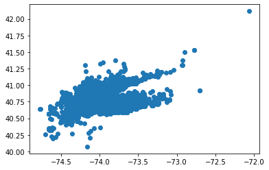
To cluster this data, let's use a machine learning unsupervised algorithm called k-means clustering. The idea behind this approach is to divide all the data samples into several groups of equal variance. Essentially, it takes in the number of clusters n_clusters (8 by default) and separates the data accordingly. To figure out the optimal number of clusters, a graphical elbow method is used. It includes the following steps:
- Training several models with a different number of clusters and gathering the values of WCSS (Within Cluster Sum of Squares) for each, meaning the sum of the squared distances of the observations from their closest cluster centroid.
- Plotting WCSS values against the corresponding values of the number of clusters.
- Selecting the lowest number of clusters where a significant decrease of WCSS happens.
from sklearn.cluster import KMeans

wcss = []
for i in range(1, 11):
    kmeans = KMeans(n_clusters=i, random_state=1)
    kmeans.fit(uber_data[['Lat', 'Lon']])
    wcss.append(kmeans.inertia_)

plt.figure(figsize=(12, 5))
plt.plot(range(1, 11), wcss)
plt.title('Elbow Method', fontsize=25)
plt.xlabel('Number of clusters', fontsize=18)
plt.ylabel('WCSS', fontsize=18)
plt.xticks(ticks=list(range(1, 11)),
          labels=['1', '2', '3', '4', '5', '6', '7', '8', '9', '10'])
plt.show()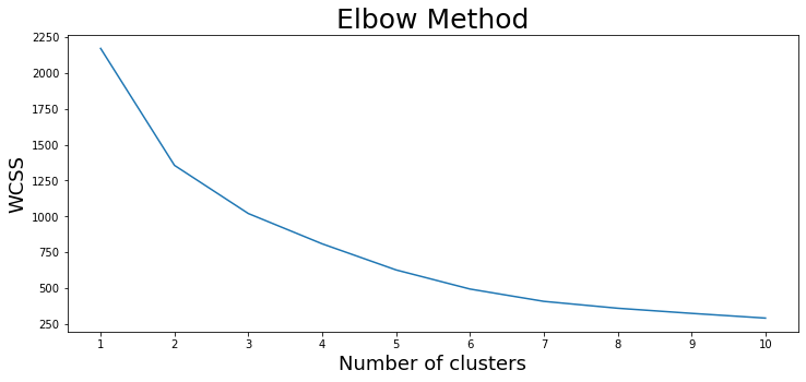
In our case, the most appropriate number of clusters seems to be 7. Let's use this value to fit a model and predict the cluster number for each pickup point. Also, we'll illustrate the data entries graphically once again, this time adding the locations of the seven cluster centroids:
kmeans = KMeans(n_clusters=7, random_state=1)
kmeans.fit_predict(df[['Lat', 'Lon']])
plt.scatter(uber_data.iloc[:, 2], uber_data.iloc[:, 1])
plt.scatter(kmeans.cluster_centers_[:, 1], kmeans.cluster_centers_[:, 0], s=100, c='lime')
plt.show()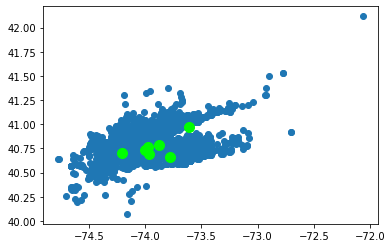
Now, we'll extract the exact coordinates for all the centroids and display them separately, without the data itself:
centroids = pd.DataFrame(kmeans.cluster_centers_)
centroids.columns = ['Lat', 'Lon']
print(centroids)
plt.scatter(centroids['Lon'], centroids['Lat'])
plt.show()
Lat Lon
0 40.688588 -73.965694
1 40.765423 -73.973165
2 40.788001 -73.879858
3 40.656997 -73.780035
4 40.731074 -73.998644
5 40.700541 -74.201673
6 40.971229 -73.611288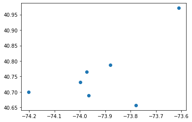
It would be more illustrative to show these centroids on a New York City map:
import folium

centroids_values = centroids.values.tolist()
nyc_map = folium.Map(location=[40.79659011772687, -73.87341741832425], zoom_start=50000)
for point in range(0, len(centroids_values)):
    folium.Marker(centroids_values[point], popup=centroids_values[point]).add_to(nyc_map)
nyc_map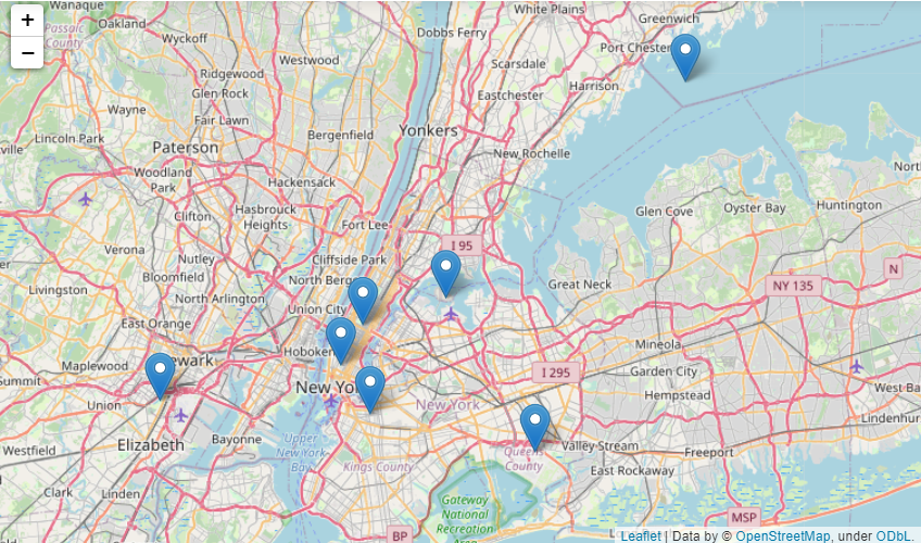
Using our model, we can predict the closest cluster for any location in New York expressed in geographical coordinates. In practical terms, it means that Uber will send an available taxi from the nearest location and serve the customer faster.
Let's find the closest cluster for Lincoln Center for the Performing Arts in the borough of Manhattan:
lincoln_center = [(40.7725, -73.9835)]
kmeans.predict(lincoln_center)array([1])And for Howard Beach in the borough of Queens:
howard_beach = [(40.6571, -73.8430)]
kmeans.predict(howard_beach)array([3])As potential ways forward, we can consider applying other machine learning clustering algorithms, analyzing different slices of data (by hour/day of the week/month), finding the most and least loaded clusters, or figuring out the relationships between the identified clusters and the Base variable from the dataframe.
Other common data science use cases in transport and logistics:
- dynamic price matching supply-demand
- forecasting demand
- automation of manual operations
- self-driving vehicles
- supply chain visibility
- damage detection
- warehouse management
- customer sentiment analysis
- customer service chatbots
Data Science in Telecom
In the last couple of decades, telecommunication technologies have grown at an incredibly fast pace and entered a new stage of their development. Nowadays, we're surrounded by electronic devices of all kinds, and many people have become literally dependent on the Internet, particularly on social networks and messengers. Sometimes this device addiction is criticized for substituting real face-to-face communication. However, we have to admit that telecom made our lives significantly easier, allowing us to connect with people all around the world in a matter of a few seconds.
This became especially true in the period of the COVID-19 pandemic when a lot of companies and schools adopted remote working or learning schemes. In such a rapidly changing reality, the quality and smoothness of digital connectivity assumed unprecedented importance in all spheres. Lockdown times made it necessary for people to call and text their colleagues, relatives and friends much more often than before. All these new tendencies led to an immense escalation in the volumes of telecommunications, which in turn resulted in generating vast amounts of data in this industry.
Using data science methods to work through the accumulated data can help the telecom industry in many ways:
- streamlining the operations,
- optimizing the network,
- filtering out spam,
- improving data transmissions,
- performing real-time analytics,
- developing efficient business strategies,
- creating successful marketing campaigns,
- increasing revenue.
Let's explore in more detail a common data science task in telecommunications, related to detecting and filtering out unwanted messages.
Data science use case in telecom: Building a spam filter
Spam filtering is a vital function of all modern written communication channels since it protects us from being bombarded with daily emails trying to scam us of our money. Technically, it's another example of a classification problem: based on the historical data, each new input message is labeled as ham (i.e., a normal message), and then it arrives directly to the recipient, or as spam, and then it's blocked or arrives into the spam folder.
A popular supervised machine learning algorithm for this purpose is the Naive Bayes classifier. It's based on the homonymous theorem from probability theory, while "naive" stays for the underlying assumption that all the words in each message are mutually independent. This assumption is not exactly correct since it ignores the inevitable existence of natural word embeddings and context. However, in the majority of low-data text classification tasks, this approach seems to work well and make accurate predictions.
There are several versions of the Naive Bayes classifier, each one with its own applicability cases: multinomial, Bernoulli, Gaussian, and flexible Bayes. The best type for our case (spam detection) is the multinomial Naive Bayes classifier. It's based on discrete frequency counts of the categorical or continuous features representing word counts in each message.
Let's apply multinomial Naive Bayes spam filtering to SMS Spam Collection Data Set from UCI Machine Learning Repository.
import pandas as pd

sms_data = pd.read_csv('SMSSpamCollection', sep='\t', header=None, names=['Label', 'SMS'])
print(f'Number of messages: {sms_data.shape[0]:,}\n\n'
      f'{sms_data.head()}')
Number of messages: 5,572
Label SMS
0 ham Go until jurong point, crazy.. Available only ...
1 ham Ok lar... Joking wif u oni...
2 spam Free entry in 2 a wkly comp to win FA Cup fina...
3 ham U dun say so early hor... U c already then say...
4 ham Nah I don't think he goes to usf, he lives aro...There are 5,572 human-classified messages. How many of them (in %) are spam?
round(sms_data['Label'].value_counts()*100/len(sms_data)).convert_dtypes()ham 87
spam 13
Name: Label, dtype: Int6413% of SMS were manually identified as spam.
To prepare the data for the multinomial Naive Bayes classification, we first have to complete the following steps:
- Encode labels from string to numeric format. In our case the labels are binary, hence we'll encode them as 0/1.
- Extract the predictor and target variables.
- Split the data into train and test sets
- Vectorize strings from the SMS column of the predictor train and test sets to obtain CSR (compressed sparse row) matrices.
The 4th step needs some more detailed explanation. Here we create a matrix object, fit it with the vocabulary dictionary (all the unique words from all the messages of the predictor train set with their corresponding frequencies), and then transform the predictor train and test sets to matrices. The result will be two matrices for the predictor train and test sets, where the columns correspond to each unique word from all the messages of the predictor train set, the rows to the corresponding messages themselves, and the values in the cells to the word frequency count for each message.
from sklearn.model_selection import train_test_split
from sklearn.feature_extraction.text import CountVectorizer

# Encoding labels
sms_data = sms_data.replace('ham', 0).replace('spam', 1)

X = sms_data['SMS'].values
y = sms_data['Label'].values

X_train, X_test, y_train, y_test = train_test_split(X, y, test_size=0.2, random_state=1)

# Vectorizing strings from the 'SMS' column
cv = CountVectorizer(max_df=0.95)
cv.fit(X_train)
X_train_csr_matrix = cv.transform(X_train)
X_test_csr_matrix = cv.transform(X_test)
Next we'll build a multinomial Naive Bayes classifier with the default parameters and check its accuracy:
from sklearn.naive_bayes import MultinomialNB
from sklearn.metrics import accuracy_score, f1_score

clf = MultinomialNB()
clf.fit(X_train_csr_matrix, y_train)
predictions = clf.predict(X_test_csr_matrix)

print(f'Model accuracy:\n'
      f'Accuracy score: {accuracy_score(y_test, predictions):.3f}\n'
      f'F1-score:       {f1_score(y_test, predictions):.3f}\n')
Model accuracy:
Accuracy score: 0.990
F1-score: 0.962As a result, we obtained a highly accurate spam filter.
Potential ways forward here can be to try other methods of train/test splitting to improve the process of vectorization by adjusting some of its numerous parameters (e.g., the cut-off for too frequent words in both spam and ham messages), and to check those very rare cases where the classifier detected a message wrongly and try to understand why it happened. In addition, we can visualize the most frequent words in spam and ham messages using a method such as a word cloud (after preliminary data cleaning and excluding all the stopwords or low-informative words). Finally, we can apply other machine or deep learning algorithms (support vector machines, decision trees, neural networks) and compare the results with the Naive Bayes approach.
Other common data science use cases in telecom:
- customer segmentation
- product development
- call detail record analysis
- recommendation systems
- customer churn rate prediction
- targeted marketing
- fraud detection
- network management and optimization
- increased network security
- price optimization
- customer lifetime value prediction
Data Science Case Studies: Courses
We have come a long way so far and explored in detail numerous applications of data science in different fields. If now you feel inspired to learn more data science use cases based on real-world datasets and to be able to apply your new knowledge and technical skills to solve practical tasks in your own sphere, you may find the following beginner-friendly short courses on various data science case studies helpful:
- Case Study: School Budgeting with Machine Learning in Python. In this course based on a case study from a machine learning competition on DrivenData, you'll explore a problem related to school district budgeting and how to make it easier and faster for schools to compare their spending with others. Applying some natural language techniques, you'll prepare the school budgets and build a model to automatically classify their items, starting with a simple version and gradually proceeding to a more advanced one. In addition, you'll be able to see and analyze the solution of the competition's winner, as well as view the other participants’ submissions.
- Analyzing Marketing Campaigns with pandas. Pandas is the most popular library of Python, and developing solid skills with its toolkit is a must for any data scientist. In this highly practical course, you'll build on Python and pandas fundamentals (adding new columns, merging/slicing datasets, working with date columns, visualizing results in matplotlib) using a fake marketing dataset on an online subscription business. You'll practice translating typical marketing questions into measurable values. Some of the questions that you'll answer are: "How did this campaign perform?", "Why is a particular channel underperforming?", "Which channel is referring the most subscribers?", etc.
- Analyzing US Census Data in Python. In this course, you'll learn how to easily navigate the Decennial Census and the annual American Community Survey and extract from them various demographic and socioeconomic data, such as household income, commuting, race, and family structure. You'll use Python to request the data for different geographies from the Census API and the pandas library to manipulate the collected data and get meaningful insights from it. In addition, you'll practice mapping with the geopandas library.
- Case Study: Exploratory Data Analysis in R. This short course will be ideal for you if you already have some basic knowledge of data manipulation and visualization tools in R. Learning the materials of this course, you'll try your skills in action on a real dataset to explore the historical voting data of the United Nations General Assembly. In particular, you'll analyze tendencies in voting between countries, across time, and among international issues. This case study will allow you to conduct a start-to-finish exploratory data analysis, gain more practice with the dplyr and ggplot2 packages, and learn some new skills.
- Human Resources Analytics: Exploring Employee Data in R. R is known for being better adapted for statistical analysis than Python. In this course, you'll leverage this advantage of R to manipulate, visualize, and perform statistical tests on a series of HR analytics case studies. Data science techniques appeared in the human resources sector relatively recently. However, nowadays they represent a very promising direction since many companies are counting more and more on their HR departments to provide actionable insights and recommendations using the database of their employees.
- Data-Driven Decision Making in SQL. In this course, you'll learn how to use SQL to support decision making and report results to management. The case study of interest is focused on an online movie rental company with a database about customer data, movie ratings, background information on actors, etc.. Some of the tasks will be to apply SQL queries to study customer preferences, customer engagement, and sales development. You'll learn about SQL extensions for online analytical processing that helps obtain key insights from complex multidimensional data.
Whether you want to become a high-level expert in data science, or your intention is just to learn useful coding skills to extract valuable data-driven insights in your own field of study, the resources above are a great place to start.
Conclusion
In summary, in this article, we have investigated what data science is from many angles, how it differs from data analytics, in which spheres it's applicable, what a data science use case is, and a general roadmap to follow to successfully solve it. We discussed exactly how data science can be useful for real-life tasks in some in-demand industries. While outlining many existing and potential applications, we focused on the most common use cases in each of those popular fields and demonstrated how to resolve each of them using data science and data analytics algorithms. If you’d like to learn more about use cases in other industries, check out our use case articles in banking, marketing, and sales. Finally, we reviewed several useful online courses for diving deeper into some other data science case studies.
One last curious observation: None of the sectors that we have considered in this work are brand new. Indeed some of them, like medicine and sales, have existed for centuries. During their entire history, much before our new era of global digitalization started, the data from those industries was also collected in one form or another; written in books and documents, and kept in archives and libraries. What has really changed dramatically in recent years with the advent of new technologies, is the fundamental understanding of the immense potential hidden in any data, and the vital importance of registering, collecting, and storing it appropriately. Applying these efforts and constantly improving data management systems has made it possible to accumulate big data in all industries for further analysis and forecasting.