Understanding Multi-Head Attention in Transformers

Introduction to the Self-Attention Mechanism

The attention mechanism, or more specifically, the self-attention mechanism, was first introduced in the famous  “Attention is All You Need“ paper by Vaswani et al. in 2017. 

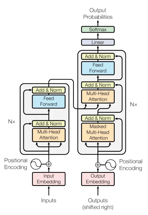
This mechanism is what powers the Transformers model, which in turn powers some of the most powerful models we have, such as LLMs and VLMs. 

So yes, it is quite important!

But here’s the thing: many people (and I used to be one of them!) believe that attention was invented in 2017.

It wasn’t.

The original attention mechanism was first introduced in 2015, when Bahdanau et al. introduced it in the context of machine translation. Their idea was to let the decoder focus on different parts of the input sentence at each decoding step, instead of relying on a single fixed context vector.

That small shift made a huge difference — and planted the seed for what would become self-attention and eventually multi-head attention.

But you might have a question at this point:

“What does attention actually mean?”

Let me introduce this concept with two simple sentences:

• “The cat sat on the mat.” → Our model might focus attention from sat to both cat and mat.
• “She drank her tea because she was thirsty.” → Attention from drank points to both tea and thirsty, connecting cause and action.

From these examples, we can start to see what attention is trying to do. It is all about focus; helping the model decide which other words are relevant to the one it's processing, often based on semantic meaning or grammatical relationships.

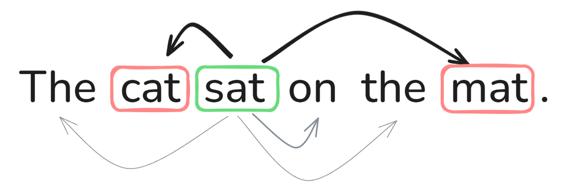
An important thing to note is that all of the tokens are used when computing the attention weights and scores (more on this later), not just some specific tokens, as can be seen in the above diagram. This also means that there will be stronger attention between some words as compared to others, as depicted by the boldness of the arrows.

This is what makes transformers so good at understanding language; they use attention to dynamically relate every word to every other word.

Intermediary steps

We have now uncovered what attention is, but we still do not know how the internal processing is.

This is where Queries, Keys, and Values (commonly abbreviated as Q, K, and V) come in. For the rest of this article, we are going to stick with our example sentence - “the cat sat on the mat”. 

Firstly, when a sentence is inputted into the Transformer, it is immediately tokenized by a tokenizer, a famous tokenizer being Byte-pair encoding. 

We can think of tokenization as splitting a text into smaller units. Since all of the words in our sentence are quite small, for this example, we can assume that each unit is equal to a word. Visually speaking, the sentence after being passed through the tokenizer should look like this:

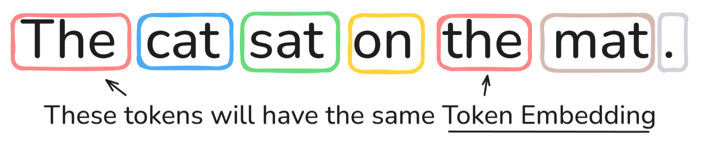
Please note that even the punctuation (full stop) has been converted into a Token. Again, for simplicity’s sake, we are assuming that the full stop is its own separate token. 

After tokenization, we use a tokenizer vocabulary to convert each token to its respective Token ID. The tokenizer vocabulary can be thought of as a database/table which holds all of the tokens that the model can identify and their respective Token ID.

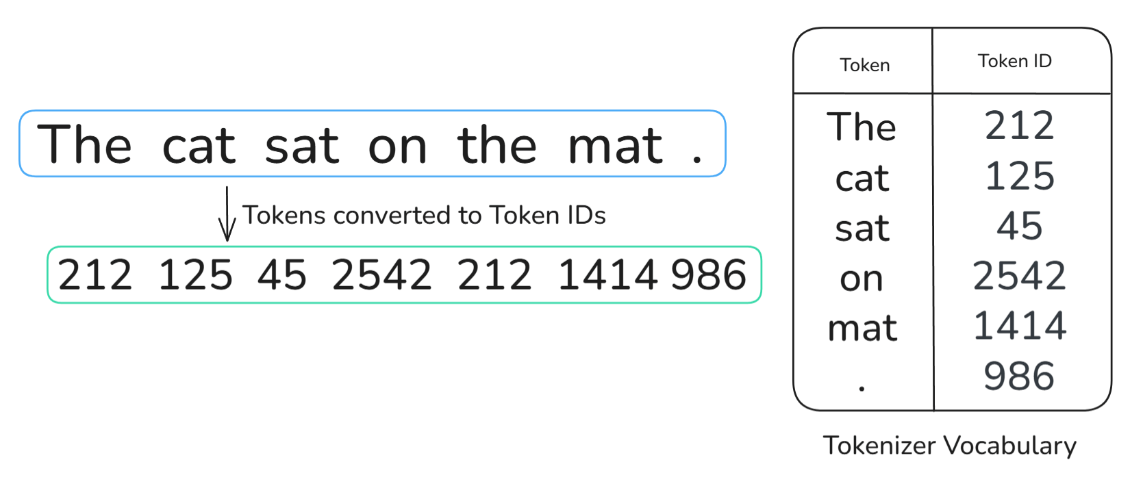
After, each of these unique token IDs are mapped to their respective token embedding using an embedding matrix. It is important to note that all of these token embeddings will be vectors of the same dimension; in our example, we are assuming 512.

The last remaining step is the addition of positional embedding so that the model has positional information of each of the tokens. The two common methods are:

1. Sinusoidal encoding (used in the original Transformer)
2. Learned position embeddings (used in BERT, GPT)

The underlying mechanics of these positional embeddings are beyond the scope of this tutorial. All we need to know for now is that we have obtained our input vectors through this formula:

Input vector = Token Embedding + Positional Embedding

Queries, keys, and values

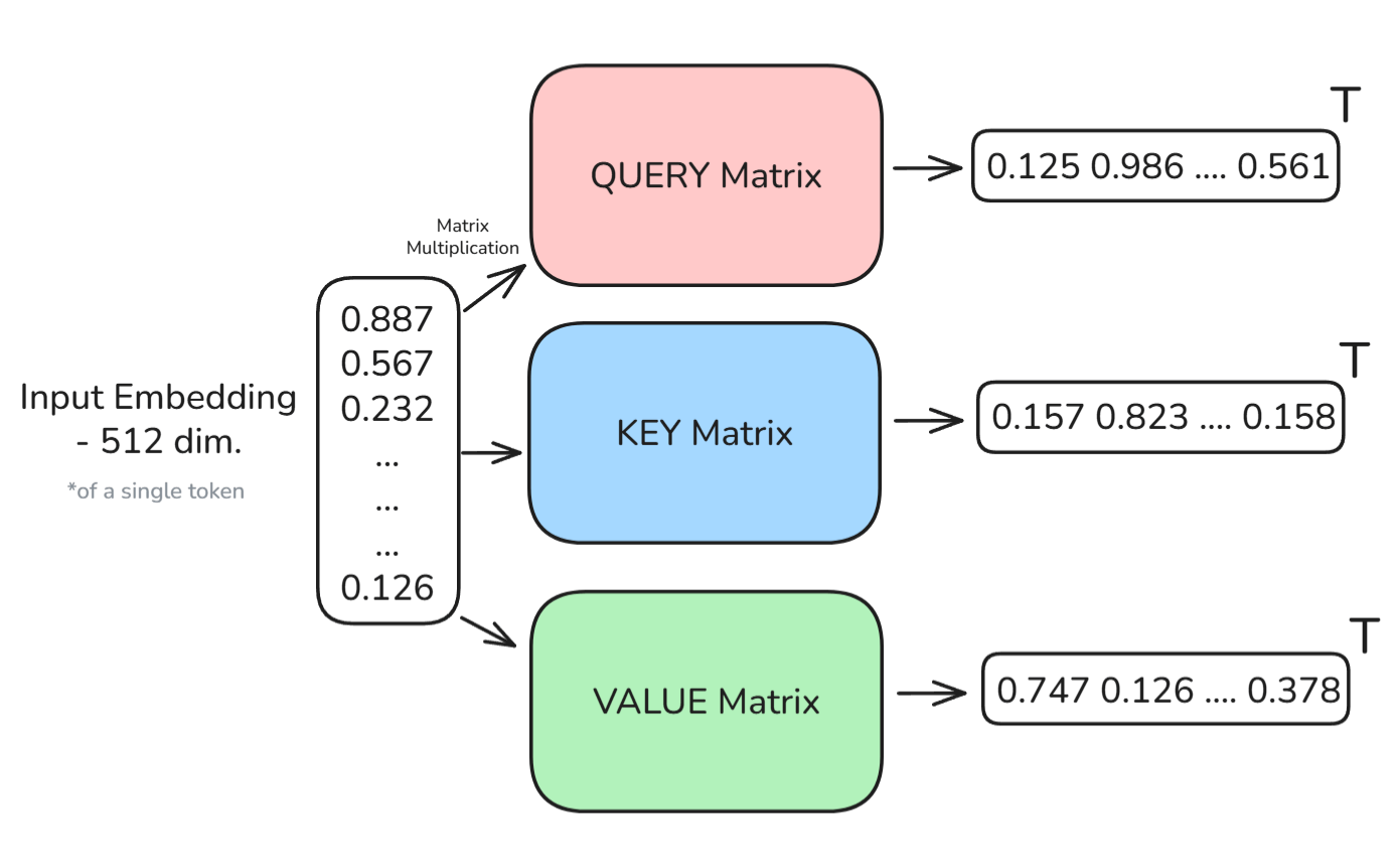
We are now finally ready to introduce Q,K,V Vectors. To begin, note that for each word in the input, we create three vectors:

• Query (Q) – this is what the word is looking for
• Key (K) – this is what the word offers to others
• Value (V) – this is the actual information the word holds

These are learnable transformations and are also their respective matrices. Mathematically, these transformations are written as this:

From this, each token can be represented by three new vectors. I have created the diagram below to help visualize this process:

Calculating scaled dot-product 

In the “Attention is all you need” paper, a mathematical formula was given, showing how the new vectors are used to calculate the Attention Weights. Let’s walk through this step by step, assuming we are calculating the Attention Weights when we are on “sat”:

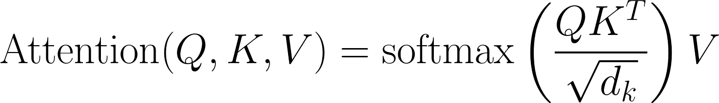
To start, we use the Query vector of “sat” to compare against the Key vectors of every other word — including itself. The result is a set of similarity scores (these are scalar) that tell us how relevant each word is to “sat”. These are more formally known as Attention Scores.

These scores are then scaled through the sqrt(d_k) to keep the scores from getting too large and helping stabilize gradients when training via backpropagation. These scaled scores are then passed through a softmax, turning them into attention weights. 

The softmax gives us a probability that tells the model how much weight to give to each word, and therefore the attention weights for a particular token will be equal to 1. 

Finally, we take a weighted sum of the value vectors, using these attention weights. 

This gives us a new vector that represents “sat” in context, enriched by the information of all of the token, but mainly from cat, mat, and any other relevant tokens.

This process happens for every token in the sentence. Each token attends to every other token, and even to itself. That’s why we call it self-attention.

Please also note that we computed the new enriched vector for a single token, but in practice, we would do this for many, if not all, of the tokens in one go, since matrix multiplication is extremely efficient. 

We can do this since the architecture is fully parallelizable. Unlike recurrent neural networks (RNNs) that process sequentially, this mechanism lets Transformers process all tokens at once, making them fast and powerful.

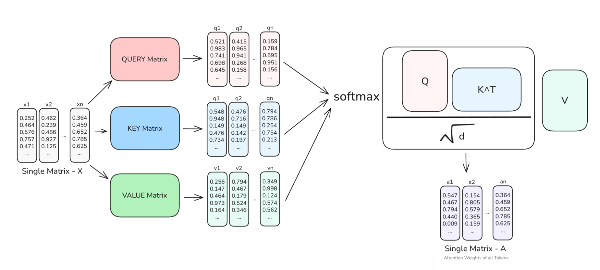
To help visualize things, take a look at the above diagram. You can see that the input matrix X is transformed to the respective Query, Ke, and Value matrices, and then the scaled dot-product attention formula is applied, to obtain the full enriched embedding vectors of all of the tokens in our input - A.

Implementing scaled dot-product attention in PyTorch

Now let’s code what we just discussed in PyTorch. Surprisingly, it is quite easy:

import torchimport torch.nn.functional as Fdef scaled_dot_product_attention(Q, K, V):    d_k = Q.size(-1)  # the dimension of the key vectors    scores = torch.matmul(Q, K.transpose(-2, -1)) / torch.sqrt(torch.tensor(d_k, dtype=torch.float32))    attn_weights = F.softmax(scores, dim=-1)    output = torch.matmul(attn_weights, V)    return output, attn_weights

By implementing a simple function, we can replicate the above discussion! Here are the most important points:

• Q, K, and V are tensors of shape [batch_size, seq_len, dim]
• The output is a new set of vectors where each token is represented in the context of the entire sequence
• Attention Scores are the raw unnormalized similarities
• Attention Weights are the normalized (via softmax) to focus and sum to 1

Different Types of Attention

There is, however, one important detail which I haven’t stated yet. See, there isn’t just one kind of attention in the Transformer - there are actually three:

1. Encoder self-attention
2. Decoder self-attention
3. Encoder–decoder (cross) attention

Each of these plays a slightly different role, so let's quickly go through them.

Encoder self-attention

This is what we have explored so far, in which in the encoder, each token attends to every other token in the same input sequence, such as “the cat sat on the mat.” example. 

The important thing to note here is that there is no restriction since the whole input is known in advance, allowing the model to build deep contextual representations of each token, where it understands what comes before and after. 

Please also note that this is happening in the encoder. 

Decoder self-attention

This is where things get slightly more difficult. Since we are now in the decoder, we don’t want each token to see the future, since that would be cheating during text generation.

Let’s take another example of “The dog barked very loudly.” When the model is generating “barked” (assuming each word is a token for simplicity reasons), it should not know that the next token is “very”, otherwise the model would not be learning to generate new tokens. 

To solve this problem, we apply a causal mask (sometimes also called a triangular mask) where it makes sure that each token can only attend to itself and the tokens before it, never the ones ahead.

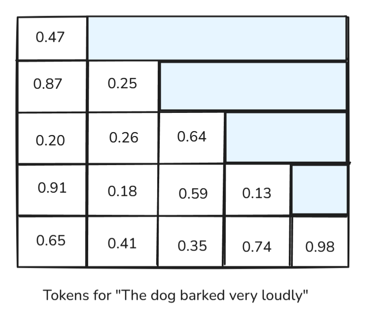
From the above diagram, we can see that the future attention scores are removed by masking them, allowing the model to learn to generate new, accurate, and sensible tokens.

Encoder-decoder (cross) attention

Once the decoder has started generating, it still needs the information from the original input (which is the thing it is responding to). This is where cross attention comes in.

Here, the decoder attends to the output of the encoder. So while decoder self-attention is masked, cross-attention is not, and so the decoder is allowed to look at all encoder tokens at once.

When I was learning this concept, I really liked the Translation Example. Pretend you are translating “Bonjour tout le monde” to English, the decoder should be able to look at all the French words as it decides on each English word right? 

This is exactly what cross attention does. However, we will not be covering cross attention in any more depth here, since it is not required for the scope of this article.

The Need for Multi-Head Attention

So now we understand how self-attention works. But now you might have this question:

If we already have attention, why do we need multiple heads of it?

For this, I would like to present the flashlight analogy, which helped build my intuition when I was first learning.

Think of a single attention head as one flashlight trying to illuminate the important parts of a sentence. But a sentence will have multiple different kinds of relationships to understand: subject-verb, object-pronoun, adjective-noun, long-range dependencies, etc.

Wouldn’t it be better if we could capture more of these relationships rather than just a single one each time?

Therefore, the solution would be to give the model multiple flashlights, each focusing on different parts of the sentence. This is multi-head attention.

Instead of computing one set of Q, K, V, and running a single attention calculation, we split the embeddings into smaller parts and run multiple independent attention heads in parallel. 

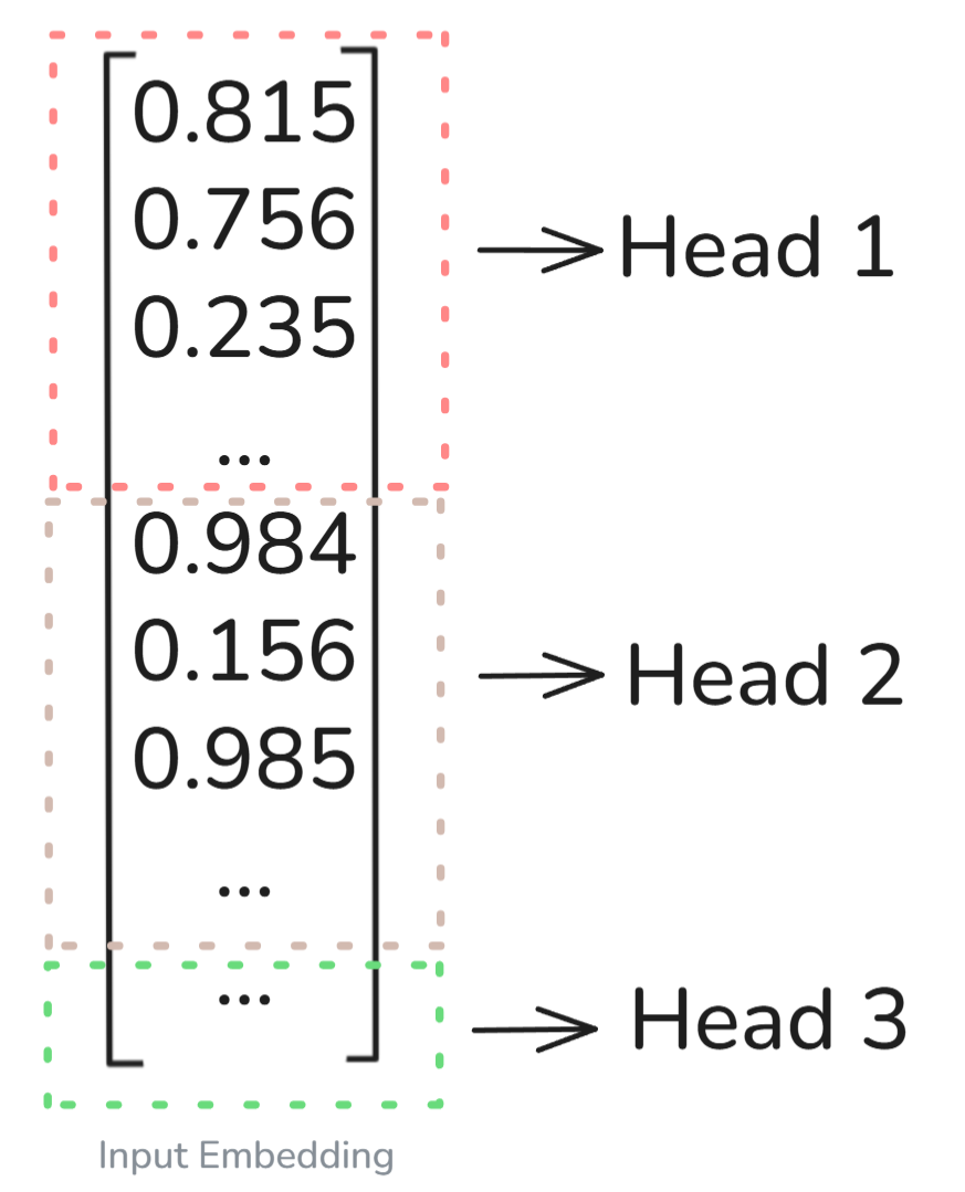
As can be seen in the above diagram, the input embedding (for a single token in this case, to make it simple) has been split evenly across the n different heads. 

In our example, let's assume that the dimension was 512 and the number of heads was 8, therefore, each attention head will process (512/8=64) dimensions in parallel, trying to capture the different relationships. 

To build your intuition further about what kinds of relationships might (I say might because we still don’t fully understand what relationship each head looks at), these heads process, let’s walk through a simple example:

Let’s consider this sentence:

“The quick brown fox jumps over the lazy dog.”

• One head might focus on adjective–noun pairs: “quick → fox”, “lazy → dog”
• Another head might focus on subject–verb: “fox → jumps”
• And another head might capture long-distance relationships: “jumps → over → dog”

The main thing to note is that all these heads run simultaneously, and their outputs are concatenated and projected back to the original embedding size (in our case 512). 

Visualizing multiple heads through code

To completely solidify our understanding on Multiple-Head Attention, let’s use the HuggingFace library to see how the Multi-Head Attention mechanism is working. 

!pip install transformers bertviz torch

First, run the above code cell to download all of the relevant packages.

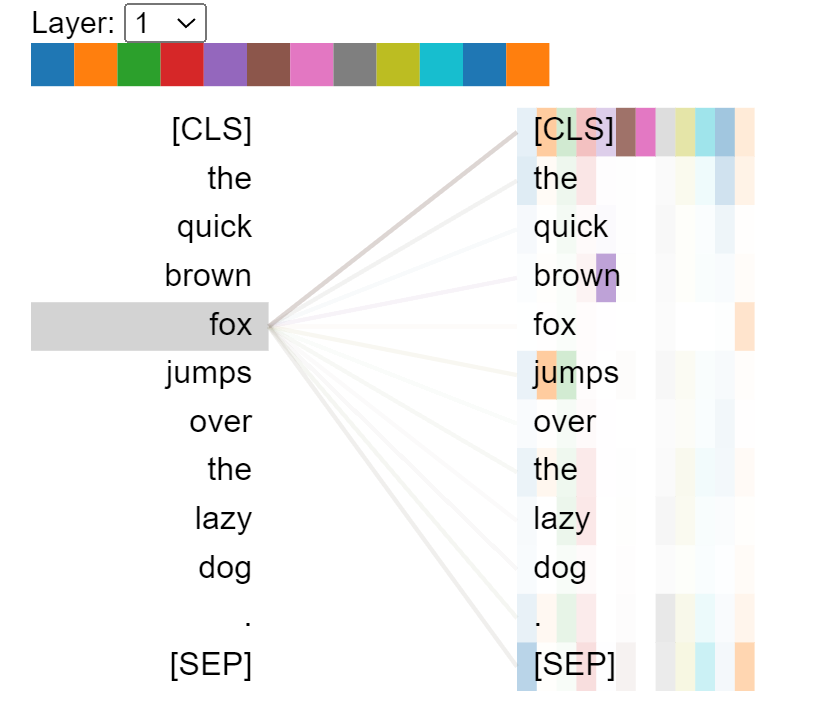
from transformers import BertTokenizer, BertModelfrom bertviz import head_viewimport torchmodel_name = 'bert-base-uncased' # We will be using the Bert modelmodel = BertModel.from_pretrained(model_name, output_attentions=True)tokenizer = BertTokenizer.from_pretrained(model_name)model.eval() # As we are not training, we have set the model to evaluation mode so no updates are made# This is our input sentencesentence = "The quick brown fox jumps over the lazy dog."# Using the tokenizer to convert the sentence into tokensinputs = tokenizer(sentence, return_tensors='pt')input_ids = inputs['input_ids']# Forward pass with attentionswith torch.no_grad():    outputs = model(**inputs)    attentions = outputs.attentions  # Tuple of (num_layers, batch, num_heads, seq_len, seq_len)# Here we decode the tokens tokens = tokenizer.convert_ids_to_tokens(input_ids[0])head_view(attentions, tokens) # Visualization

The output we get can be seen below. Notice how there are 12 different colours, which means there are 12 Heads in this model. The thickness of the lines also correlates with the magnitude of the attention scores between the tokens. 

Implementing Multi-Head Attention: Best Practices

In this section, we are going to be writing the pseudocode for the Multi-Head Attention mechanism. Let’s first assume that our input: X has the shape [batch, seq_len, d_model]. 

Then we can proceed with the pseudocode: 

Q = X @ W_Q # Calculating the Query valuesK = X @ W_K # Calculating the Key valuesV = X @ W_V# Calculating the Value valuesQ_i, K_i, V_i = split_into_heads(Q, K, V, num_heads) # Now we split the Q,K,V into multiple different heads (by evenly splitting the dimensions)# Here we compute scaled dot-product attention for each headscores = (Q_i @ K_i.T) / sqrt(head_dim)scores += maskA_i = softmax(scores)A_i = dropout(A_i)Z_i = A_i @ V_iZ = concat_heads(Z_i) # We have to concatenate all of the Heads# This is our final linear projection matrixoutput = Z @ W_Ooutput = dropout(output)

All of this should be familiar to you by now, except for maybe the final linear projection matrix. 

Let’s quickly go over this. 

After all the individual attention heads finish their work, their outputs are concatenated back into a single vector. But this combined output still needs to be reshaped into the original model dimension and this is where the final linear projection matrix comes in. It simply maps the concatenated output back to the same size as the input embedding, so it can be passed to the next layer in the Transformer.

Let’s also discuss some of the optimizations and best practices:

1. Parallelization: Since each head is independent, we can compute them all in parallel.
2. Matrix multiplication: We batch everything using linear algebra operations (e.g. matmul), which is highly optimized.
3. FlashAttention (Advanced): This is a newer technique that uses low-level CUDA tricks to reduce memory overhead and speed up attention — especially on long sequences.

In terms of best practices, when we are coding up the attention layer, there are 3 main hyperparameters we should look at:

1. num_heads: How many attention heads to run in parallel, where we have to make sure it divides evenly into d_model.
2. head_dim: Dimension of each head.
3. dropout_rate: To prevent overfitting.

Conclusion

We covered a lot in this article. We started off with a simple idea: attention is about focus. Then, we explored how Transformers use this focus by calculating how each word relates to every other word using Queries, Keys, and Values.

We saw how self-attention (and briefly other Attention such as Causal and Cross Attention) gives each token a rich, context-aware representation. And then we took it a step further with multi-head attention, where instead of relying on just one "flashlight", we give the model multiple, each capturing different patterns in the sentence, all at once.

This is what gives Transformers their real power. They don’t just read; they understand the underlying structure, meaning, and relationships across entire sequences. 

Now, in this article, we have covered one aspect of Transformers, but there is still quite a lot to learn, so check out this full, detailed course: Transformer Models with PyTorch Course. 

If you want to jump into the applications side, I would also recommend going for the Developing Multi-Input Models For OCR project or the Working with HuggingFace course. If you prefer articles, then check out this intuitive Complete Guide to Building a Transformer Model with PyTorch and my other guide on Vision Transformers.