Softmax Activation Function in Python: A Complete Guide

Activation functions are the backbone of neural networks. They are important components that introduce non-linearity and enable these networks to learn complex patterns. The softmax activation function is important, particularly when dealing with multi-class classification problems.

While alternatives like Sigmoid and ReLU have their specific use cases, softmax is better at handling situations where outputs must be interpreted as probabilities across mutually exclusive classes.

The softmax activation function transforms an entire vector of numbers into a probability distribution. This unique characteristic makes it indispensable for tasks where we need to classify inputs into one of several possible categories.

From image recognition systems that identify thousands of object categories to natural language processing models that predict the next word in a sentence, softmax provides the mathematical foundation for making decisions across multiple possibilities.

In this article, we'll look at what the softmax activation function is, how it works mathematically, and when you should use it in your neural network architectures. We'll also look at the practical implementations in Python.

What is the Softmax Activation Function?

The Softmax activation function is a mathematical function that transforms a vector of raw model outputs, known as logits, into a probability distribution. In simpler terms, it takes a set of numbers and converts them into probabilities that sum up to 1.

Unlike some activation functions that operate on individual values independently, softmax works on an entire vector of values, transforming them collectively into a probability distribution where all elements sum to exactly 1.

In the context of neural networks, softmax is typically applied to the final layer of a network designed for multi-class classification. When we have multiple possible categories and need our model to indicate the probability of each category, the softmax activation function is the standard choice.

How does the softmax function work?

The raw outputs from a neural network's final layer are often called "logits." These values can range from negative infinity to positive infinity and don't have a direct probabilistic interpretation. The softmax activation function transforms these logits into a more interpretable form by:

1. Taking the exponential of each input value (which ensures all values are positive).
2. Dividing each exponential by the sum of all exponentials (which ensures the outputs sum to 1).

This transformation is crucial because it allows us to interpret the network's output as a probability distribution. For example, if a neural network is classifying images into three categories (cat, dog, bird), the softmax output might be [0.7, 0.2, 0.1], indicating a 70% probability for cat, 20% for dog, and 10% for bird.

The softmax activation function plays a vital role in creating valid probability distributions because:

• It ensures all output values are between 0 and 1.
• It guarantees that all outputs sum to exactly 1.
• It preserves the ranking of input values (larger inputs result in larger probabilities).
• It accentuates differences between larger values while suppressing differences between smaller values.

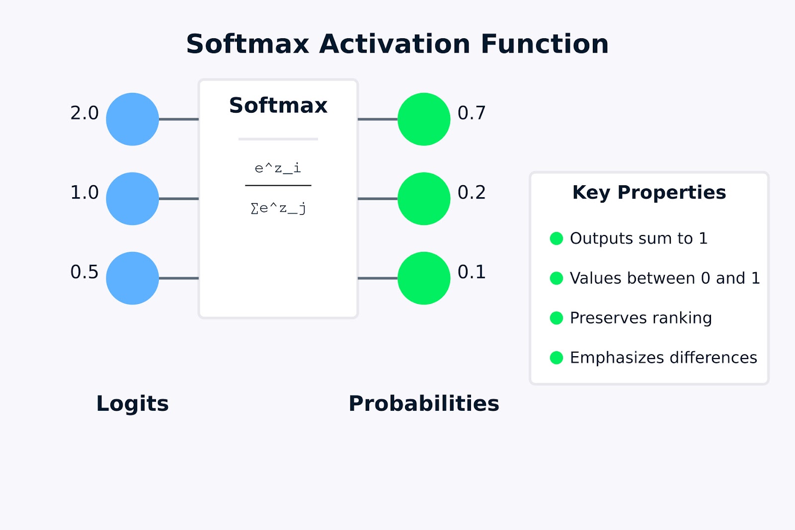
Softmax Activation Function

The above visualization shows how the softmax activation function transforms raw logits (the input values 2.0, 1.0, and 0.5) into a probability distribution (0.7, 0.2, and 0.1). The formula inside the softmax box represents how each output probability is calculated by taking the exponential of an input value and dividing it by the sum of all exponentials. 

The key properties highlighted on the right indicate why softmax is useful for multi-class classification problems. In the next section, we’ll look at the mathematical formula and how it works.

Softmax Activation Function Formula and How It Works

Now that we understand what the softmax activation function is, let's look at the mathematical formulation and how it transforms inputs into probability distributions.

The softmax activation function formula can be expressed mathematically as:

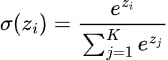
Where:

• ​z_i is the input value (logit) for class i
• e^z_i is the exponential function applied to z_i (also written as exp(z_i ​))
• K is the total number of classes
• The denominator sums the exponentials of all input values, ensuring the output values sum to 1

The softmax activation function follows these steps to transform a vector of inputs into a probability distribution:

1. Calculate exponentials: First, we compute the exponential (e^x) of each input value. This step ensures all values are positive, as e^x > 0 for any real number x
2. Sum the exponentials: We calculate the sum of all the exponential values from step 1.
3. Normalize: We divide each exponential value by the sum calculated in step 2. This normalization ensures that all outputs are between 0 and 1 and sum to exactly 1.

Let's apply the softmax activation function formula to a simple example to see how it works in practice.

Suppose we have a neural network with three output neurons for a three-class classification problem (e.g., identifying whether an image contains a cat, dog, or bird). After the final computation, the network outputs the following logits: z = [2.0, 1.0, 0.5].

To convert these logits into probabilities using the softmax function:

1. Calculate exponentials:
• e^2.0 = 7.389
• e^1.0 = 2.718
• e^0.5 = 1.648
2. Sum the exponentials:
• 7.389 + 2.718 + 1.648 = 11.755
3. Normalize:
• P(class 1) = 7.389 / 11.755 ≈ 0.628 or 62.8%
• P(class 2) = 2.718 / 11.755 ≈ 0.231 or 23.1%
• P(class 3) = 1.648 / 11.755 ≈ 0.140 or 14.0%

The resulting probability distribution [0.628, 0.231, 0.140] sums to 1, with the highest probability assigned to the class corresponding to the highest logit value. This example demonstrates how the softmax activation function preserves the ranking of input values while transforming them into a valid probability distribution.

Notice how the original input values (2.0, 1.0, 0.5) maintained their relative ranking in the output probabilities, but the differences between them were accentuated. This property makes softmax particularly useful in classification tasks where we want to identify the most likely class with confidence.

In the next section, we’ll look at the different ways to implement the softmax activation function using Python.

Implementing Softmax Activation Function in Python

Now that we understand the theory behind the softmax activation function, let's see how to implement it in Python. We'll start by writing a softmax function from scratch using NumPy, then see how to use it with popular deep learning frameworks like TensorFlow/Keras and PyTorch.

Writing softmax from scratch using NumPy

Before diving into frameworks, it's important to understand how to implement the softmax activation function from scratch. This helps build intuition for what's happening under the hood.

import numpy as np

def softmax(x):
    """
    Compute softmax values for each set of scores in x.
    
    Args:
        x: Input array of shape (batch_size, num_classes) or (num_classes,)
        
    Returns:
        Softmax probabilities of same shape as input
    """
    # For numerical stability, subtract the maximum value from each input vector
    # This prevents overflow when calculating exp(x)
    shifted_x = x - np.max(x, axis=-1, keepdims=True)
    
    # Calculate exp(x) for each element
    exp_x = np.exp(shifted_x)
    
    # Calculate the sum of exp(x) for normalization
    sum_exp_x = np.sum(exp_x, axis=-1, keepdims=True)
    
    # Normalize to get probabilities
    probabilities = exp_x / sum_exp_x
    
    return probabilities

This implementation follows the softmax activation function formula exactly, with one important addition: we subtract the maximum value from each input vector before exponentiation. 

This "shifting" operation doesn't change the mathematical result but helps prevent numerical overflow, which can occur when computing exponentials of large numbers.

Let's test our implementation with a simple example:

# Sample logits from a neural network (batch of 2 examples, 3 classes each)
logits = np.array([
    [2.0, 1.0, 0.5],  # First example
    [3.0, 2.0, 1.0]   # Second example
])

probabilities = softmax(logits)
print("Logits:\n", logits)
print("\nSoftmax probabilities:\n", probabilities)
print("\nSum of probabilities (should be 1 for each example):", np.sum(probabilities, axis=1))

Output:

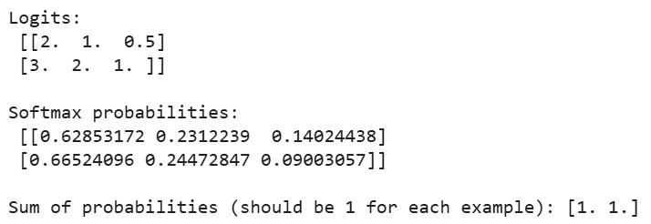
When we run the above code, we’ll see that the sum of probabilities for each example equals 1, confirming that our softmax implementation produces valid probability distributions. For the first example, the largest probability corresponds to the largest logit (2.0), and similarly for the second example.

Using softmax in TensorFlow/Keras

TensorFlow and Keras make it easy to use the softmax activation function in your neural networks. Let's build a simple classifier for the MNIST dataset step by step.

First, let's import the necessary libraries and load the dataset:

import tensorflow as tf
from tensorflow.keras.models import Sequential
from tensorflow.keras.layers import Dense, Flatten, Softmax
from tensorflow.keras.datasets import mnist
import matplotlib.pyplot as plt
import numpy as np

# Load and preprocess the MNIST dataset
(x_train, y_train), (x_test, y_test) = mnist.load_data()

# Normalize pixel values to be between 0 and 1
x_train, x_test = x_train / 255.0, x_test / 255.0

# One-hot encode the labels
y_train_one_hot = tf.keras.utils.to_categorical(y_train, 10)
y_test_one_hot = tf.keras.utils.to_categorical(y_test, 10)

The MNIST dataset contains 28x28 pixel grayscale images of handwritten digits (0-9). We normalize the pixel values to be between 0 and 1 for better training dynamics, and we convert the class labels to one-hot encoding, which is the preferred format for softmax outputs.

Now, let's create a neural network model with a softmax output layer:

# Method 1: Using softmax as the activation function in the final layer
model1 = Sequential([
    Flatten(input_shape=(28, 28)),  # Convert 28x28 images to 784-length vectors
    Dense(128, activation='relu'),   # Hidden layer with ReLU activation
    Dense(10, activation='softmax')  # Output layer with softmax activation
])

# Method 2: Using a separate Softmax layer
model2 = Sequential([
    Flatten(input_shape=(28, 28)),
    Dense(128, activation='relu'),
    Dense(10),  # Linear output (logits)
    Softmax()   # Separate softmax layer
])

Here, we demonstrate two equivalent ways to incorporate the softmax activation function in a neural network:

• Method 1: Directly specifying 'softmax' as the activation function in the final Dense layer
• Method 2: Adding a separate Softmax layer after the Dense layer that outputs raw logits

Both approaches produce identical results, but the second method makes the separation between logits and probabilities more explicit, which can be useful in certain scenarios.

Next, let's compile and train the model:

# Compile the model
model1.compile(
    optimizer='adam',
    loss='categorical_crossentropy',  # This loss works well with softmax
    metrics=['accuracy']
)

# Print model summary
print("Model with softmax activation:")
model1.summary()

# Train the model
print("\nTraining the model...")
history = model1.fit(
    x_train, y_train_one_hot,
    epochs=5,
    batch_size=128,
    validation_split=0.1,
    verbose=1
)

Output:

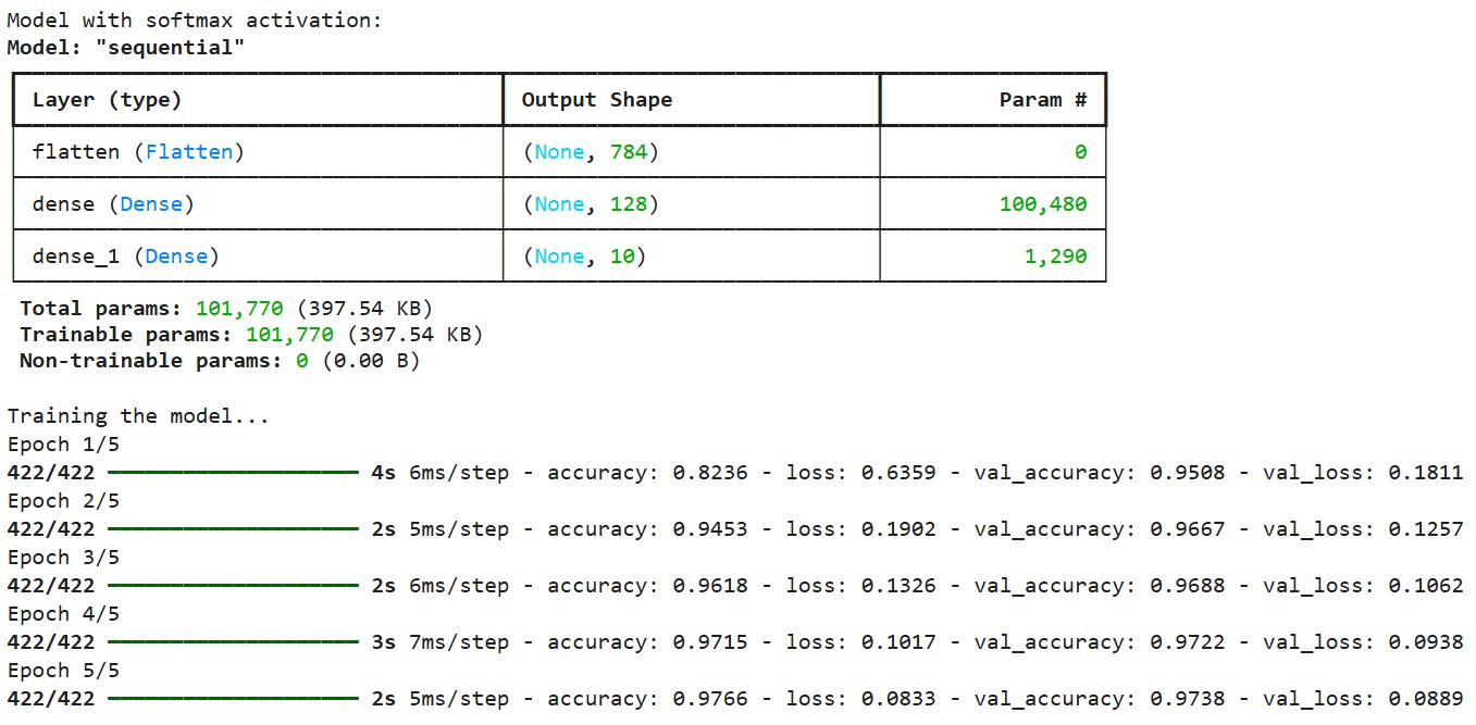We compile the model using the categorical cross-entropy loss function, which is designed to work with softmax outputs. This loss function measures the difference between the predicted probability distribution and the true one-hot encoded labels. We use the Adam optimizer, which adaptively adjusts the learning rate during training.

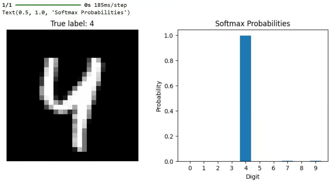
After training, we can use the model to make predictions and visualize the results:

# Let's check predictions on a sample
sample_idx = 42
sample_image = x_test[sample_idx]
true_label = y_test[sample_idx]

# Get model predictions (probabilities across all classes)
predictions = model1.predict(sample_image[np.newaxis, ...])

# Visualize the results
plt.figure(figsize=(10, 4))

# Plot the image
plt.subplot(1, 2, 1)
plt.imshow(sample_image, cmap='gray')
plt.title(f"True label: {true_label}")
plt.axis('off')

# Plot the probability distribution
plt.subplot(1, 2, 2)
plt.bar(range(10), predictions[0])
plt.xticks(range(10))
plt.xlabel('Digit')
plt.ylabel('Probability')
plt.title('Softmax Probabilities')

This code selects a test image, passes it through the trained model, and visualizes both the image and the resulting probability distribution from the softmax output. The highest bar in the probability plot represents the model's prediction.

Output:

TensorFlow also provides a built-in function for applying softmax directly:

# Demonstrate using a custom softmax function in TensorFlow
def custom_softmax(logits):
    """Custom implementation of softmax in TensorFlow"""
    exp_logits = tf.exp(logits - tf.reduce_max(logits, axis=-1, keepdims=True))
    return exp_logits / tf.reduce_sum(exp_logits, axis=-1, keepdims=True)

# Example usage of custom softmax
logits = tf.constant([[2.0, 1.0, 0.5], [3.0, 2.0, 1.0]])
custom_probs = custom_softmax(logits)
tf_probs = tf.nn.softmax(logits)

print("\nCustom softmax:", custom_probs.numpy())
print("TensorFlow softmax:", tf_probs.numpy())

Output:

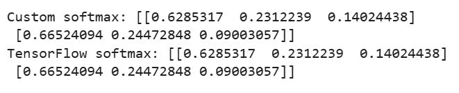
This example compares a custom implementation of softmax with TensorFlow's built-in tf.nn.softmax() function. Both should produce identical results. The custom implementation also includes the numerical stability trick of subtracting the maximum value before exponentiation.

Using Softmax in PyTorch

Now, let's implement a similar model using PyTorch and the CIFAR-10 dataset. We'll start with importing libraries and setting up the data, as shown below:

import torch
import torch.nn as nn
import torch.optim as optim
import torchvision
import torchvision.transforms as transforms
import matplotlib.pyplot as plt
import numpy as np

# Set the device
device = torch.device("cuda:0" if torch.cuda.is_available() else "cpu")
print(f"Using device: {device}")

# Load and preprocess the CIFAR-10 dataset
transform = transforms.Compose([
    transforms.ToTensor(),
    transforms.Normalize((0.5, 0.5, 0.5), (0.5, 0.5, 0.5))  # Normalize RGB channels
])

# Load a small subset of the CIFAR-10 dataset for demonstration
trainset = torchvision.datasets.CIFAR10(root='./data', train=True,
                                        download=True, transform=transform)
trainloader = torch.utils.data.DataLoader(trainset, batch_size=64,
                                          shuffle=True, num_workers=2)

testset = torchvision.datasets.CIFAR10(root='./data', train=False,
                                       download=True, transform=transform)
testloader = torch.utils.data.DataLoader(testset, batch_size=64,
                                         shuffle=False, num_workers=2)

# Define the class names for CIFAR-10
classes = ('plane', 'car', 'bird', 'cat', 'deer',
           'dog', 'frog', 'horse', 'ship', 'truck')

The above code sets up PyTorch to use GPU acceleration if available, loads the CIFAR-10 dataset (which contains 32x32 color images across 10 classes), and prepares data loaders for training and testing.

Next, let's define a simple convolutional neural network as shown below:

# Define a simple convolutional neural network
class SimpleCNN(nn.Module):
    def __init__(self):
        super(SimpleCNN, self).__init__()
        # Convolutional layers
        self.conv1 = nn.Conv2d(3, 16, 3, padding=1)
        self.conv2 = nn.Conv2d(16, 32, 3, padding=1)
        self.pool = nn.MaxPool2d(2, 2)
        
        # Fully connected layers
        self.fc1 = nn.Linear(32 * 8 * 8, 128)
        self.fc2 = nn.Linear(128, 10)  # 10 classes in CIFAR-10
        
        # Activation functions
        self.relu = nn.ReLU()
        
        # Note: We don't define softmax here as it will be applied with the loss function
    
    def forward(self, x):
        # Convolutional layers with ReLU and pooling
        x = self.pool(self.relu(self.conv1(x)))  # -> 16x16x16
        x = self.pool(self.relu(self.conv2(x)))  # -> 8x8x32
        
        # Flatten the output
        x = x.view(-1, 32 * 8 * 8)
        
        # Fully connected layers
        x = self.relu(self.fc1(x))
        x = self.fc2(x)  # Raw logits output
        
        # Note: No softmax here, as PyTorch's CrossEntropyLoss applies it internally
        return x

This CNN processes the 32x32 RGB images through convolutional layers, applies ReLU activation and pooling, and ends with fully connected layers. Notably, the model does not include a softmax layer in its forward pass. Instead, it outputs raw logits.

This is a common pattern in PyTorch because the CrossEntropyLoss function used during training internally applies softmax before computing the loss, which is more numerically stable. 

Let's also see how to explicitly include softmax if needed:

# Applying softmax within the model
class ModelWithSoftmax(nn.Module):
    def __init__(self):
        super(ModelWithSoftmax, self).__init__()
        self.features = SimpleCNN()
        self.softmax = nn.Softmax(dim=1)
    
    def forward(self, x):
        logits = self.features(x)
        probabilities = self.softmax(logits)
        return probabilities

We define two model variants: SimpleCNN outputs raw logits, while ModelWithSoftmax explicitly applies softmax to produce probabilities. For training, we use SimpleCNN with CrossEntropyLoss, which is the standard approach in PyTorch.

Let's define a training function:

# Create the model and move it to the device 
model = SimpleCNN().to(device) 
# Define loss function and optimizer 
criterion = nn.CrossEntropyLoss()  # Combines LogSoftmax and NLLLoss 
optimizer = optim.SGD(model.parameters(), lr=0.001, momentum=0.9)
# Train the model (only a few epochs for demonstration)
def train_model(epochs=2):
    for epoch in range(epochs):
        running_loss = 0.0
        for i, data in enumerate(trainloader, 0):
            inputs, labels = data[0].to(device), data[1].to(device)
            
            # Zero the parameter gradients
            optimizer.zero_grad()
            
            # Forward + backward + optimize
            outputs = model(inputs)  # These are logits (pre-softmax)
            loss = criterion(outputs, labels)
            loss.backward()
            optimizer.step()
            
            running_loss += loss.item()
            if i % 100 == 99:
                print(f'[{epoch + 1}, {i + 1}] loss: {running_loss / 100:.3f}')
                running_loss = 0.0
    
    print('Finished Training')

Finally, let's create a function to visualize model predictions:

# Function to display predictions with softmax probabilities
def show_prediction_example():
    # Get a batch of test images
    dataiter = iter(testloader)
    images, labels = next(dataiter)
    
    # Select a single image
    img = images[0].to(device)
    label = labels[0]
    
    # Get the model's prediction (logits)
    with torch.no_grad():
        logits = model(img.unsqueeze(0))
    
    # Apply softmax to get probabilities
    probabilities = torch.nn.functional.softmax(logits, dim=1)
    
    # Plot the image and probabilities
    fig, (ax1, ax2) = plt.subplots(1, 2, figsize=(10, 4))
    
    # Show the image
    img_np = img.cpu().numpy()
    img_np = np.transpose(img_np, (1, 2, 0))
    # Denormalize the image for display
    img_np = img_np * 0.5 + 0.5
    ax1.imshow(img_np)
    ax1.set_title(f"True label: {classes[label]}")
    ax1.axis('off')
    
    # Show the probabilities
    probs = probabilities[0].cpu().numpy()
    ax2.bar(range(10), probs)
    ax2.set_xticks(range(10))
    ax2.set_xticklabels(classes, rotation=45)
    ax2.set_xlabel('Class')
    ax2.set_ylabel('Probability')
    ax2.set_title('Softmax Probabilities')
    
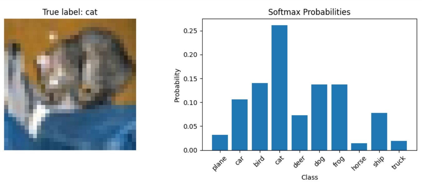
    plt.tight_layout()

This function demonstrates how to get softmax probabilities from a trained model during inference. It passes an image through the model to get logits, applies softmax manually using torch.nn.functional.softmax(), and then visualizes both the image and the resulting probability distribution.

Now, let’s train the model:

train_model()

Output:

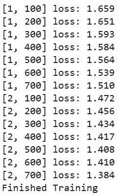
Let’s predict and see how the probabilities show up for a test image:

show_prediction_example()

Output:

In the next section, we'll look at the specific scenarios where softmax is the optimal choice, examine when softmax activation function should be used, and discuss real-world applications in various deep learning models.

When to Use the Softmax Activation Function?

Understanding when to use the softmax activation function is important for designing effective neural networks. The softmax activation function finds its primary application in the output layer of neural networks designed for classification tasks.

Softmax for multi-class classification

Softmax is the standard choice when our model needs to classify inputs into one of several mutually exclusive categories. Common examples include:

• Image classification (identifying objects in photos)
• Document categorization (assigning topics to text)
• Named entity recognition (identifying person names, locations, etc.)
• Speech recognition (mapping audio to text)

Probabilistic interpretation and confidence scores

When we need our model to output probabilities rather than just class predictions, softmax provides a probabilistic interpretation of the model's confidence across all possible classes.

Softmax in reinforcement learning and attention mechanisms

In reinforcement learning and sequential decision problems, softmax can be used to convert action values into a probability distribution for action selection.

Modern transformer-based architectures use softmax to distribute attention across different parts of the input sequence.

The strong mathematical foundation and intuitive probabilistic interpretation make the softmax activation function particularly well-suited for classification problems where classes are mutually exclusive.

Deep learning models

Several deep learning architectures use the softmax activation function. 

Image classification networks like ResNet, VGG, and Inception all use softmax in their final layer to classify images into thousands of categories. For example, models trained on ImageNet typically have a 1000-unit softmax layer corresponding to 1000 object categories.

In language modeling, RNN-based models use softmax to predict the next word in a sequence from a vocabulary that might contain tens of thousands of words.

Modern NLP architectures like BERT, GPT, and T5 use softmax in multiple components:

• In attention mechanisms to determine how much focus to place on different parts of the input
• In the final classification layer for tasks like sentiment analysis or document classification

Variational Autoencoders (VAEs) and certain Generative Adversarial Networks (GANs) use softmax in their discriminator components or for categorical latent variable modeling.

In the next section, we’ll look at the differences between the softmax activation function and the sigmoid activation function.

Softmax vs Sigmoid Activation Function

The sigmoid function, defined as σ(x) = 1/(1+e^(-x)), transforms a single real number into a value between 0 and 1. In contrast, the softmax activation function operates on a vector of numbers, converting them into a probability distribution.

Here are the fundamental differences between these two activation functions:

Input and output dimensions

• Sigmoid: Takes a single scalar input and produces a single scalar output between 0 and 1.
• Softmax: Takes a vector of n inputs and produces a vector of n outputs that sum to 1.

Probability interpretation

• Sigmoid: Output represents the probability of a single binary event (e.g., "Is this email spam?").
• Softmax: Outputs represent probabilities across multiple mutually exclusive classes (e.g., "Which digit from 0-9 is this?").

Independence of outputs

• Sigmoid: When used across multiple neurons, each output is independent of others. Multiple outputs can all be high or all be low.
• Softmax: Outputs are interdependent—if one probability increases, others must decrease to maintain a sum of 1.

Mathematical relationship

Interestingly, the sigmoid function is actually a special case of the softmax activation function when there are only two classes. This is why sigmoid is often called "binary softmax."

When to use softmax vs when to use sigmoid

Choosing the right activation function is crucial for ensuring a neural network outputs meaningful predictions, and the decision between softmax and sigmoid depends on the nature of the classification task.

Use sigmoid when:

• Solving binary classification problems (two classes)
• Each output needs to be interpreted independently
• Implementing multi-label classification where an instance can belong to multiple classes simultaneously
• Creating attention mechanisms or gates in recurrent neural networks

Use softmax when:

• Dealing with multi-class classification problems (more than two classes)
• Classes are mutually exclusive (an input belongs to exactly one class)
• You need a proper probability distribution across all possible outcomes
• Implementing the final layer of most image classification networks

For instance, in a neural network that classifies images of handwritten digits (0-9), the softmax activation function would be appropriate for the output layer since each image represents exactly one digit. On the other hand, for a network that detects multiple objects in an image (e.g., "contains person", "contains car", "contains tree"), sigmoid activations would be more suitable since multiple objects can be present simultaneously.

Here's a quick reference table comparing the softmax vs sigmoid activation function:

Understanding the distinction between these activation functions is critical for designing effective neural networks. While the softmax activation function is the go-to choice for multi-class classification problems, sigmoid remains valuable for binary classification and problems requiring independent probabilities.

In the next section, we’ll look at the common issues that arise and the considerations to be made while working with softmax activation functions.

Common Issues and Considerations

When working with the softmax activation function in your deep learning models, several challenges can affect model performance and reliability. Understanding these issues and knowing how to address them will help you build more robust models.

Numerical stability challenges

Numerical stability is a critical concern when using the softmax activation function. The exponential operation in the softmax activation function formula can lead to numerical overflow or underflow if not handled properly.

For instance, when dealing with very large input values (like 1000 or higher), the exponential function produces extremely large numbers that can exceed the maximum representable floating-point value in your system. This leads to overflow errors, producing "infinity" values that make the final division operation yield undefined results (NaN - Not a Number).

The standard solution, as mentioned in our implementation section, is to subtract the maximum value from all inputs before applying the exponential function. This shift doesn't change the relative proportions after normalization but keeps the values within a manageable range. 

Modern deep learning frameworks handle this issue internally, but it's important to understand the problem when implementing custom operations or debugging unexpected behavior.

Softmax and overconfidence in predictions

Another common issue with the softmax activation function is that neural networks tend to become overconfident in their predictions, even when they're wrong. This overconfidence occurs because:

1. The exponential nature of softmax amplifies small differences in logits.
2. Modern deep neural networks are powerful enough to memorize training data perfectly.
3. Cross-entropy loss continues to push probabilities toward 1 for correct classes, even after a model reaches good accuracy.

In practice, this means a model might assign a 99% probability to a prediction that's actually incorrect. This can be problematic in critical applications where reliable uncertainty estimation is essential. For example, a medical diagnosis system that's overconfident in incorrect predictions could lead to inappropriate treatment decisions.

The gap between a model's confidence (from softmax probabilities) and its actual accuracy is known as calibration error. Well-calibrated models produce confidence scores that match their accuracy rates—if a model predicts events with 80% confidence, those events should occur approximately 80% of the time.

Regularization Techniques to Improve Performance

Fortunately, several techniques can help address these issues with the softmax activation function:

Temperature scaling

Temperature scaling introduces a parameter T that controls the "softness" of the probability distribution. By dividing the logits by this temperature parameter before applying softmax, you can adjust how peaked or uniform the resulting distribution becomes.

Higher temperatures (T > 1) produce softer probability distributions with less extreme values, which can help reduce overconfidence. Lower temperatures (T < 1) make the distribution more peaked toward the highest value. Temperature scaling is commonly used as a post-processing technique after training to calibrate model confidence without affecting the model's ranking of classes.

Label smoothing

Label smoothing replaces hard one-hot target vectors with slightly smoothed distributions. Instead of training the model to output exact zeros and ones, label smoothing encourages the model to be slightly less confident by targeting values like 0.9 for the correct class and 0.025 for incorrect classes (in a 4-class problem).

By training with these smoothed labels, the model learns to be less confident in its predictions, which improves generalization and makes the model more robust to label noise. This technique has become standard practice in many state-of-the-art image classification models.

Dropout and ensemble methods

Using dropout during training and keeping it enabled during inference (a technique called Monte Carlo dropout) allows you to sample multiple predictions for the same input and estimate uncertainty. If the model produces consistent predictions across multiple forward passes with different dropout patterns, it's likely more certain about its prediction.

Similarly, ensemble methods combine predictions from multiple models to improve performance and provide better uncertainty estimates. The disagreement between models in an ensemble can serve as a measure of uncertainty.

Calibration techniques

Platt scaling and other calibration methods can be applied after training to ensure that the confidence scores from softmax actually correspond to true probabilities. These methods typically use a validation set to learn parameters that map the original model outputs to well-calibrated probabilities.

For example, a simple temperature scaling approach (as mentioned earlier) can be optimized on validation data to minimize calibration error. More complex approaches include isotonic regression and Bayesian binning.

The softmax bottleneck

Recent research has identified a fundamental limitation of the softmax function known as the "softmax bottleneck." This refers to the fact that the expressivity of softmax-based language models is limited by the rank of the weight matrix in the final layer. In natural language contexts with complex dependencies, this can prevent models from fully capturing the underlying conditional distributions.

Advanced architectures like Mixture of Softmaxes (MoS) have been proposed to address this limitation by using a weighted combination of multiple softmax distributions.

By being aware of these common issues and implementing appropriate solutions, you can improve the reliability and performance of models that use the softmax activation function for classification tasks.

Conclusion

The softmax activation function is an essential component of neural networks for multi-class classification problems, transforming raw logits into interpretable probability distributions. We've explored its mathematical foundation, implementation in Python, comparison with sigmoid, practical use cases, and techniques for addressing common challenges like numerical instability and overconfidence.

Ready to deepen your understanding of neural networks? 

• Explore our Introduction to Activation Functions tutorial or dive into framework-specific courses on Deep Learning With Keras and PyTorch.
• To learn about other important activation functions, check out our article on ReLU and start building more effective neural networks today!