Vision Transformers (ViT) Tutorial: Architecture and Code Examples

We all know that Transformers have become foundational in natural language processing and are now gaining traction in computer vision. Vision Transformers (ViTs) offer a novel approach to image understanding by using the same principles used in text-based models; Large Language Models.

ViTs were first introduced in 2020 by Google Research in the paper “An Image is Worth 16×16 Words,” showing that transformers trained on large image datasets can match or beat CNNs. Since then, practical variants like DeiT and Swin have broadened their use across many vision tasks.

In this tutorial, I will guide you through the core concepts, architectural components, and practical applications of vision transformers (the vanilla/original variant). By the end, we will understand not just how ViTs work, but also how to implement them in our own computer vision projects. I also recommend checking out my other guide on multi-head attention.  

What is a Vision Transformer (ViT)?

Let’s begin by gently introducing vision transformers. 

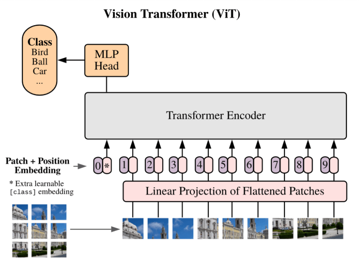
These models treat an image as a sequence of data, similar to how a language model processes words in a sentence. Then the image is divided into fixed-size patches, each of which is flattened and embedded into a vector. 

These vectors are then passed through a standard transformer encoder, which models the relationships between patches globally using the attention mechanism. 

Comparison with convolutional neural networks

This is fundamentally different from convolutional neural networks (CNNs), which focus on local features and rely on hierarchical feature extraction.

Since we are speaking about CNNs, let’s talk about what the differences are between them and ViTs:

Obviously we haven’t covered vision transformers in full depth yet but it is useful to go over some of the points which might not make sense from the get go. 

For example, inductive bias and receptive fields are terms which are important but you might have not heard of before. 

Inductive bias explanation

Inductive Bias means the assumptions a model makes to help it learn from data. This seems quite confusing but it should make sense after reading this analogy.

Imagine we are doing a jigsaw puzzle together. We can think the pieces will connect based on shape and colour. This assumption helps us place the pieces together faster. This is how a CNN model works. 

It makes smart guesses by assuming that nearby parts in an image are related, like how puzzle pieces close to each other often belong to the same part of the picture. It also assumes that if we move a shape around, it’s still the same shape. These helpful guesses are called strong inductive biases.

Now imagine we’re given a big pile of puzzle pieces, but we have no idea what the final image looks like. We don’t even know if we should look at shape or colour or maybe something else entirely. So we start trying everything and slowly figure out what works.

That’s what a Transformer model does. It doesn’t make strong assumptions. It learns patterns by looking at a lot of data. This is called minimal inductive bias. It gives the model more freedom but needs more data and time to learn.

Receptive field explanation

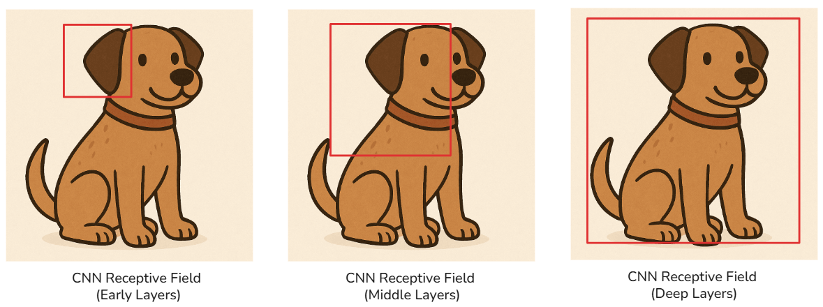
The above image now shows how the receptive field of a CNN model changes. Remember, there are multiple convolutional layers in a CNN, and so as we go deeper into the network, each layer’s neuron is influenced by a progressively larger region of the input. 

This expanding receptive field allows deeper layers to detect more complex and global features, as shown in the figure above (from ear to face to whole dog). 

This is quite different from a Vision Transformer’s receptive field:

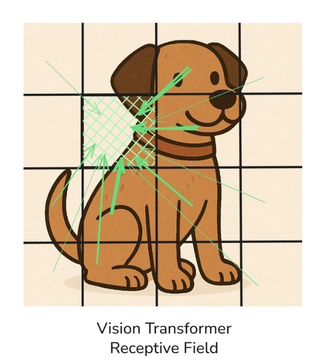
In the above illustration, we can see that the receptive field in a (vanilla) ViT is global, so all of the patches attend to each other by different magnitudes (shown by the thickness of the arrows). 

For simplicity, I have shown that the patch (coloured in green) is being attended to by the other patches, but in reality, all of the patches will attend to each other (it would have been too messy to draw!)

When to use CNNs vs vision transformers

Understanding when to use a CNN versus a vision transformer is quite important for making effective architectural choices in our computer vision workflows. 

Both models have their strengths (and weaknesses!), but they perform better under different conditions depending on data size, computational resources, and the complexity of the visual patterns we are trying to model.

I like to refer to these points when trying to make the choice between them:

You should use CNNs when:

1. Working with limited data - We have already stated that CNNs come with strong inductive biases like locality, which help them generalize well even with smaller datasets. This makes them a reliable choice for tasks where collecting large volumes of labeled data is impractical.
2. Real-time performance is important - CNNs tend to have lower inference latency and are computationally more efficient on standard hardware, especially mobile and edge devices. Their architecture is optimized for performance with fewer parameters and less memory usage.
3. Compute budget is limited - Training a CNN from scratch or fine-tuning a pretrained one requires significantly fewer resources compared to ViTs. We can train a decent CNN with a single GPU and moderate memory, which is not always the case for transformer-based models.

You should use Vision Transformers when:

1. Access to large-scale labeled datasets and robust compute infrastructure - Like I mentioned in the comparison table, vision transformers are data-hungry and require significant training time and memory, especially in their vanilla form. With enough data and compute, they are capable of outperforming CNNs in many benchmarks.
2. We need to capture long-range spatial relationships - Unlike CNNs, which are local in their processing (remember the receptive field section), ViTs leverage self-attention to model relationships between all image patches, making them particularly useful for tasks where spatial context across the entire image matters.
3. Wanting to use pretrained models and transfer learning - We can access pretrained ViTs (such as through HuggingFace or timm) and so fine-tuning becomes much more practical. In this case, even mid-sized datasets can give us great results without training from scratch.

So to summarize, if you ever find yourself in a low-resource environment or need fast, dependable results with limited data, CNNs are the safer and more efficient choice. 

On the other hand, if your project demands deep global reasoning across visual space and you have the compute power to back it, vision transformers are the better option. 

Components of a Vision Transformer

Let’s now dive into the actual architecture of the Vision Transformer. Since there are multiple stages (five to be specific) to this, let’s explore them one by one. 

Stage 1: Image patching

This is the first transformation step, where we have to convert an image into a form the transformer can understand.

Let’s say we have a 224x224 image. Rather than feeding it in whole, we divide it into smaller, fixed-size patches. If each patch is 16x16 (like proposed in the original paper), then the image gets split into 14×14 = 196 patches, since (224/16 =14).

A really easy way to understand this is by thinking of cutting a photograph into perfectly equal square tiles. Each patch contains localized information and will act like a "word" in a sentence.

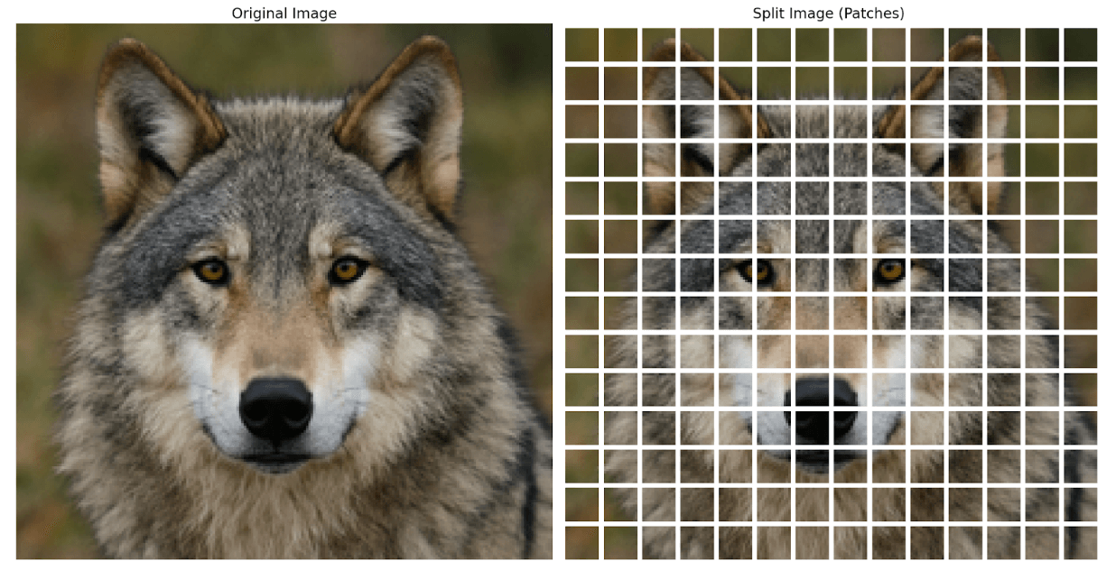
In the above illustration, you can see that the image of a wolf gets split into smaller square (and equal) patches - 196 to be exact.

You might have one question here, though:

“The image is RGB, so what happens to the 3 colour channels?”

This is an important point to note, where each patch is actually a block of data, where, in our case, it has the shape of 16x16x3. 16x16 is the height and width, and 3 is the colour channels, making each patch a 3-dimensional tensor. 

This makes each patch a compact representation of both the spatial and color information from a local region of the image.

This division into patches transforms the 2D spatial structure of the image into a 1D sequence of multi-dimensional data, suitable for a transformer model.

Stage 2: Patch embedding

Next, we need to transform each image patch into a numerical representation that the transformer can use.

Every 16x16 RGB patch is flattened into a single vector. In our example, 16×16×3 = 768 values. We are essentially unrolling all pixel and color values into a single line of numbers.

These raw vectors, while informative, are not yet in a space suitable for learning. So we pass each one through a trainable linear projection layer. Think of this as a dense layer that maps every 768-dimensional input into a new embedding space of size D (often also 768, but not always).

Why?

This projection is important because it aligns all patch tokens into a consistent, learnable format that the transformer encoder expects. Up until this point, we have had a sequence of fixed-length vectors, where each vector represents one patch of the image.

This entire process transforms spatial and color-rich patches into a unified sequence of "tokens" (analogous to word embeddings in NLP), allowing the transformer to treat the image as a structured series of learnable entities.

Stage 3: Positional encoding

There is one thing left before we send these tokens into our encoder. You might have guessed this if you have already covered LLMs before!

Transformers are inherently position-agnostic.

This means that they treat sequences of inputs as unordered collections, meaning they have no built-in mechanism to understand the order or position of tokens. And this is quite a big issue in image analysis, where both spatial structure and layout are critical!

Let’s talk about this in detail. 

In the context of images, each patch represents a specific region of the original image. If we feed the model a sequence of patch embeddings without indicating where each patch came from, it has no idea whether a patch came from the top-left corner or the bottom-right. 

This lack of spatial awareness would limit our model's ability to understand patterns, shapes, structures, etc.

To solve this, we add something called positional encoding to each patch embedding. This is a vector that acts like a spatial tag; a vector that encodes the original position of the patch within the image. These positional vectors are added directly to the patch embeddings before the sequence enters the transformer.

There are two common types of positional encodings:

• Fixed (sinusoidal) positional encoding: These use sine and cosine functions at different frequencies to encode position information. They are deterministic and do not require learning. This was also what was used in the famous “Attention is all you need” paper.
• Learned positional encoding: These are trainable parameters that the model learns during training. Each position in the sequence gets its own learnable vector.

If you are confused at this point, a really easy way to grasp this concept is by thinking of positional encodings as GPS coordinates for the patches. 

They tell the transformer the original position of the token. By including this information, we allow the self-attention mechanism to model both the content of each patch and its relative or absolute position within the image.

This step is crucial — without it, the Vision Transformer would be unable to reconstruct the structure of an image, no matter how powerful the attention mechanism is.

Stage 4: Transformer encoder block

Now we have arrived at the point where all the deep learning happens — pattern discovery, context modeling, and feature fusion.

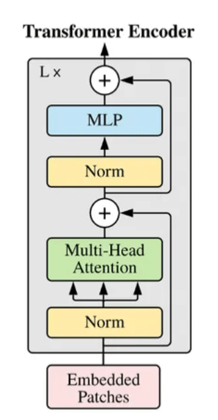
Now there are several of these Encoder blocks stacked on top of each other to make the full Vision Transformer Encoder. Let’s dive into what each encoder block contains:

• Multi-head self-attention (MHSA): This mechanism lets each patch interact with every other patch. It helps the model determine what parts of the image are most relevant to each other.
• Instead of looking at a patch in isolation, MHSA gives it a global context.
• Multiple attention heads look at different aspects of the relationships which gives a richer interpretation of the image. 
• Feedforward neural network (FFN): This is a small Multi-Layer Perceptron that processes each token independently after attention. The reason we do this is to improve the model’s ability to learn complex, nonlinear patterns.
• Residual connections and layer norm: These stabilize training and help gradients flow better through the network.

Overall, these encoder blocks are stacked in layers (e.g., 12 in ViT-Base), where with each layer, learning deeper image representations.

Stage 5: Classification token and MLP head

We are almost there! Now let's move to the last and final stage of the (vanilla) ViT. 

After all the encoder layers, we need a way to summarize everything and make a prediction.

So we introduce a special [CLS] token at the beginning of the patch sequence. This is a learnable embedding that interacts with all other tokens during encoding.

As it moves through the transformer layers, it gathers global information. At the end, we extract this token and pass it through another multilayer perceptron (MLP) head, which is usually a couple of dense layers followed by a softmax (for classification).

This final step gives us the predicted label, like saying “this image is a dog” based on the information collected by the [CLS] token. This is a very important point to note, which is that it is the [CLS token] only that is sent to this final MLP Head and therefore used for classification, not the other tokens!

Notable Vision Transformer Architectures

Let’s now look at some revolutionary Vision Transformer architectures. 

• ViT (Google Brain) - This was the original vision transformer (and the one we have been following throughout this article) that introduced the patch-based transformer model for image classification using large datasets like ImageNet-21k. 
• DeiT (Data-efficient image Transformer) - Introduced by Facebook AI, DeiT improves data efficiency by incorporating knowledge distillation techniques, enabling training on smaller datasets.
• Swin Transformer - Uses hierarchical architecture and shifted windows to reduce computation while maintaining accuracy. It is especially effective in dense prediction tasks like object detection.
• Other Variants - Models like BEiT, CvT, and MobileViT incorporate various design enhancements to improve training efficiency, model compactness, or inference speed.

Using Pre-Trained Vision Transformers 

Now, a lot of the time, we will not be training a ViT from scratch! So let’s explore how we can use pre-trained ViT models from popular deep learning libraries.

Huggingface transformers library

One of the easiest and most reliable ways to use vision transformers is through the Hugging Face Transformers library. It provides pretrained ViT models that are ready to use with just a few lines of code. 

I have written some code here to download and use the original ViT Base model:

# Imports neededfrom transformers import ViTImageProcessor, ViTForImageClassificationfrom PIL import Imageimport torchimport requests# Here I am loading and preprocessing an image - but you can use any image of your choiceimage = Image.open(requests.get(https://huggingface.co/datasets/huggingface/cats-image?image-viewer=ED6CB286C90CF5F1FAF278077DF091477DF05416', stream=True).raw)# Here, we load and process the ViT modelprocessor = ViTImageProcessor.from_pretrained('google/vit-base-patch16-224')model = ViTForImageClassification.from_pretrained('google/vit-base-patch16-224')# Preprocessing the image so it gets it into the necessary formatinputs = processor(images=image, return_tensors='pt')# Forward pass - with no backpropagationwith torch.no_grad():    outputs = model(**inputs)# Here we get the predicted labels (since we are performing classification)logits = outputs.logits	predicted_class = logits.argmax(-1) # Selects the index of the class with the highest logit score (highest predicted probability)print(f"Predicted class index: {predicted_class.item()}")

Let’s talk about this code in a bit more depth. Firstly, you might have a question about having to download two separate components. These are separate, but they are complementary to each other:

1. ViTImageProcessor – This is responsible for preprocessing the image before it is passed into the model. It handles resizing, normalization, and converting the image into the format expected by the vision transformer. The best way to think of this is as the vision equivalent of a tokenizer in NLP!
2. ViTForImageClassification – This is the actual model that performs inference. It expects inputs in a specific tensor format and outputs predictions (e.g., logits or class probabilities).

Another doubt which you could have is about output.logits and more specifically about what logits is. 

In machine learning models — especially classification models — logits are the raw output values produced by the final layer of the model before applying any activation function like softmax. They represent unnormalized scores for each class.

A good way to think about them is as the model's internal confidence levels for each class. These values can be positive or negative and are not constrained to sum to one.

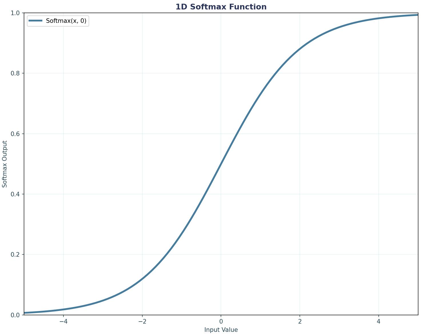
To convert logits into probabilities, we have to apply the softmax function, which scales the values into a probability distribution.

So, when we use argmax(logits, -1), we are simply selecting the index (class) with the highest raw score, which is usually equivalent to the one with the highest probability after softmax.

Using timm library

Another great and famous library for using vision transformers is timm (by Ross Wightman). It also provides a wide variety of pretrained ViT variants and is well-suited for quick experimentation or fine-tuning. Here is how we can load and use a ViT model for inference:

# Relevant importsimport timmimport torchfrom torchvision import transformsfrom PIL import Imageimport requests# Loading an imageurl = 'https://huggingface.co/datasets/huggingface/cats-image?image-viewer=ED6CB286C90CF5F1FAF278077DF091477DF05416'image = Image.open(requests.get(url, stream=True).raw)# Here we have defined the transformation we are going to do on the imagetransform = transforms.Compose([    transforms.Resize((224, 224)),    transforms.ToTensor(),    transforms.Normalize(mean=[0.5, 0.5, 0.5], std=[0.5, 0.5, 0.5])])image_tensor = transform(image).unsqueeze(0)  # Adding batch dimension# Loading the ViT modelmodel = timm.create_model('vit_base_patch16_224', pretrained=True)model.eval() # Setting it to evaluation mode# Inference componentwith torch.no_grad():    outputs = model(image_tensor)    predicted_class = outputs.argmax(dim=1) # Obtaining the class with the highest probabilityprint(f"Predicted class index: {predicted_class.item()}")

You should be able to now see the similarity between timm and the transformers library. Both provide pretrained ViT models, allow for image processing (although in timm we used standard PyTorch code), and in the end, we obtain the class with the highest logit.

Conclusion

Overall, vision transformers have reshaped computer vision by turning images into “sentences” of patches and using self-attention to capture global context from the very first layer. In this tutorial, we’ve learn about:

1. Why ViTs differ from CNNs – minimal inductive bias, global receptive fields, massive scalability, etc
2. When to choose each model – Again, CNNs excel with limited data and tight latency budgets whereas ViTs are better when we have abundant data and powerful hardware.
3. Underlying ViT architecture – We covered all of the different stages from image patching and learned positional encodings to multi-head self-attention, residual paths, and the [CLS] token for classification.
4. Practical implementation – How to load pretrained models from different libraries - Hugging Face or timm, preprocessing images, and extracting predictions.

To keep learning, I recommend you take a look at this article on How Transformers Work, which will teach you about the theory behind Transformers. To consolidate this, I then recommend exploring how to build a transformer from scratch.  

If you want to learn both at the same time while getting hands-on, then our course on Transformer Models with PyTorch is the place to go.