What Is a Linear Function? A Guide with Examples

If you’ve ever taken a math class, there is a high chance that you have bumped into a linear function early on, like in middle school algebra or while scribbling lines on graph paper.

Linear functions are everywhere in math and beyond. But many people feel like linear functions are a bit hard to understand. Even professionals sometimes gloss over the “why” behind the equations.

In this article, I will build a clear, intuitive description of linear functions and explain what makes them tick, how they’re written, and how to spot them. By the end, you will see them not as irrelevant abstract rules, but as reliable tools for understanding steady change.

The Core Idea Behind Linear Functions

At its heart, a linear function is about steady and predictable relationships.

Imagine, for instance, that you are walking at a constant speed. For every step forward that you take, you cover the same distance. This constant rate of change is the exact source of linearity that makes a linear function linear. As your input, like time or steps, increases by a fixed amount, the output, like the distance covered, shifts by the same fixed amount.

This predictability is what makes linear functions very handy. Thus, the outputs don’t leap or curve unexpectedly. They just march forward in a straight line, reliably. When you make a plot on a graph, you would trace a perfect straight line like a laser beam. It’s this simplicity that allows us to trust them for modeling the world.

A Simple Definition of a Linear Function

With the intuition in place, let’s pin it down neatly using some more mathematical formality. A linear function is a mathematical rule that maps inputs to outputs, where the change in the output is always proportional to the change in the input. In symbols, it’s often something like this:

However, we will talk about that later in this article. The most important takeaway here is that the output grows or shrinks at a steady clip, no matter where you are on the input scale.

Intuitively, A linear function is called linear because it harks back to lines. This sets linear functions apart from nonlinear ones, like for instance quadratic functions that arc upward like a rainbow or exponential ones that explode as the input grows.

The Standard Form of a Linear Function

Most of the linear functions wear their structure plainly in what is called the slope-intercept form. It looks like this:

Here, x is your input that you can think of as the variable you plug in, and y is your output. The m is the slope that tells us about the rate of change of the function or how steeply the line climbs or drops.

A bigger m means a steeper tilt and a negative one points downward. Then there’s the b, the y-intercept, which is simply the output when x is zero. The y-intercept defines your starting point on the y-axis.

In many textbooks, the notation of m and b can change to a and b, or m and p, but it will have the same outcome.

Linear Function Rate of Change

Before we label it “slope,” let’s focus on what it really means. Picture this as “how much does the output budge when the input ticks up by one unit?” If every extra hour of work nets you $20 more pay, that’s a rate of $20 per hour, which is indeed a constant change. Positive rates mean growth while negative ones mean a decline, like a cooling pie losing heat steadily.

This rate is the backbone of linearity. It does not speed up or slow to a crawl. In the language of mathematics, we call this the slope (m in our main equation), but it is the same idea.

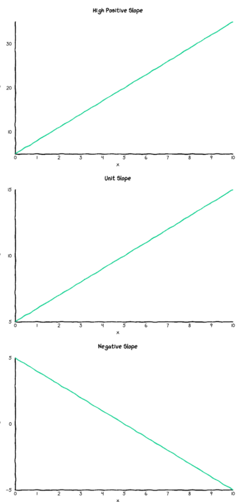
In this figure, I tried to illustrate different setups of the linear functions, keeping the b constant and playing with the m.

Linear Function Starting Value

The y-intercept b is the baseline output at zero input that you can think of as a fixed setup cost. It helps anchor the function to provide more context for how changes accumulate. 

In this figure I changed the values of b while keeping the m constant to 2.

How Linear Functions Appear on a Graph

The graphs of linear functions are straight lines due to a constant rate. Adjust the rate m so that the line tilts steeper or flatter. Shift the starting value b and the line shifts up or down while having the same tilt.

Examples of Linear Functions

There are different ways we can describe a linear function. We can describe it numerically, like f(x) = 3x + 2. This means that the outputs rise by 3 per x-increase, and y is initially 2 when x is initially 0.

We can describe it more casually, like saying the cost of something like a taxi would be equal to $3 base fare + $2 per mile. A fixed start with a steady increment.

Linear vs. Nonlinear Functions

Nonlinear relationships break the constancy as the rates vary and the graphs curve. Real relationships often approximate linear over short ranges and are useful as baselines.

This figure illustrates very well some examples of linear and nonlinear functions.

Where Linear Functions Show Up

Linear functions are the reliable backdrop for how we make sense of the world. They are our gateway for framing change as steady and scalable. Arguably, in physics, they simplify motions without friction, or in economics, they baseline the costs before complexities creep in.

In different fields, they serve as approximations because real-world data often has nearly-linear or locally-linear relationships. Biology might linearize enzyme rates over narrow ranges, and engineering linearizes stress-strain in materials. They are ubiquitous because steady change is everywhere once you look.

Linear Functions and Linear Regression

Linear regression uses data to fit a linear function as the best-fit line. It is essentially trying to estimate m and b of the equation mentioned above to find the line that fits perfectly with the collected observations. It is an approximation for the trends in scattered real data, not an actual perfection.

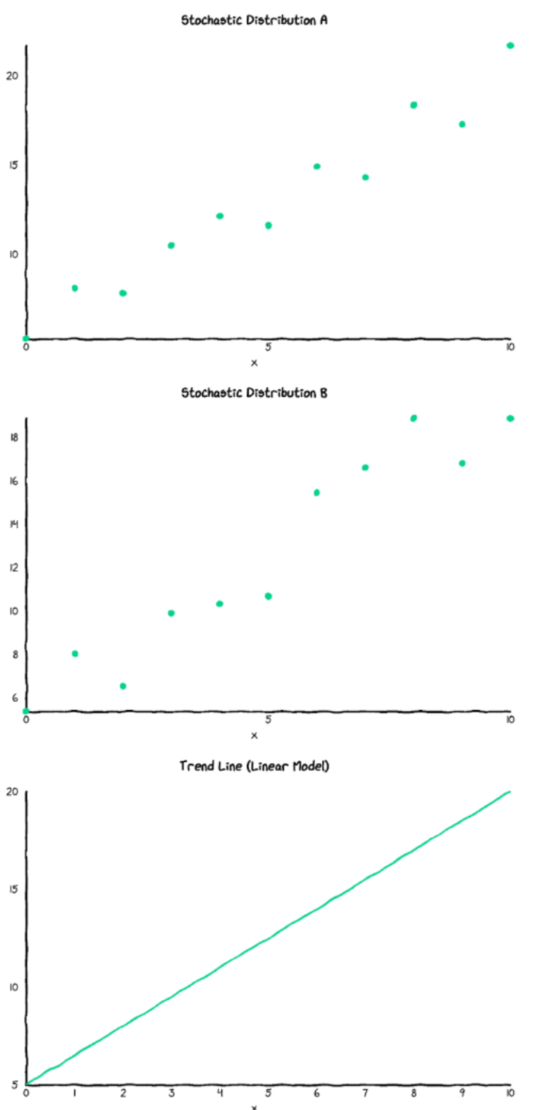
In this illustration, I showed how we can model slightly noisy real-world data points with a linear function.

Common Misunderstandings About Linear Functions

You should avoid these mistakes when thinking about linear functions:

1. Not every straight graph is linear. Lines end and sometimes change direction.
2. Real life isn’t perfectly linear. What we do is approximate it.
3. You should clearly distinguish the rate m from the start b because they shape the paths differently.

Tips for Recognizing Linear Functions

To recognize a linear function, check these rules:

• Look for constant change
• Check differences, not ratios
• Think in “per unit” terms
• Be cautious with noisy real-world data

Conclusion

Linear functions model straight-line relationships using a constant rate of change from an initial value. Because of this structure, they are simple to interpret and easy to apply. You’ll see them appear in equations, graphs, and everyday cost or estimation problems.

Keep learning with us. I recommend our Introduction to Regression with statsmodels in Python course. When you take the course, you will see how regression is more flexible than it seems. By using transformations, you will be able to model both linear and non-linear relationships using regression.