Come calcolare il tempo in Excel: guida con esempi

Potrebbe sorprenderti sapere che Excel memorizza l’ora come frazione di una giornata. Questo significa che non salva 8:30 AM così come la vedi, ma come 0.35417, cioè 8,5/24. Puoi vederlo come il 35,4% dell’intera giornata. 

In questo articolo, tratterò questi e altri scenari importanti:

• Differenza oraria: calcolare l’intervallo tra ora di inizio e ora di fine all’interno della stessa giornata.
• Tempo trascorso: misura la durata su più giorni usando timestamp completi.
• Tempo tra date: calcolare l’intervallo tra due date di calendario, in giorni, ore o minuti.
• Tempo totale: sommare più voci orarie senza incorrere nell’azzeramento a 24 ore.
• Tempo medio: calcolare la media di più voci orarie.

Come calcolare la differenza oraria in Excel

Prima o poi ti capiterà di calcolare l’intervallo tra un’ora di inizio e un’ora di fine (ora di fine - ora di inizio). Che tu usi il formato a 12 ore o a 24 ore, per Excel entrambi sono decimali. 

Il fatto che Excel esegua quel calcolo e restituisca decimali non è un problema; renderlo leggibile sì, ed è qui che entra in gioco la formattazione.

Guarda questo esempio:

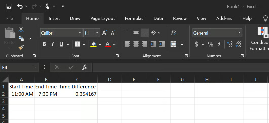
Qui, la cella C2 mostrerà per impostazione predefinita 0.354167 (8,5/24). Il numero è corretto. Rappresenta 8 ore e 30 minuti come frazione di una giornata. Per renderlo leggibile, applica il formato personalizzato [h]:mm.

Ecco, passo dopo passo, come applicare il formato corretto:

1. Seleziona la cella C2.

2. Premi Ctrl + 1 per aprire la finestra di dialogo Formato celle.

3. Fai clic su Personalizzato.

4. Nel campo Tipo, inserisci [h]:mm oppure scorri tra le opzioni e fai clic su [h]:mm:ss e poi su OK.

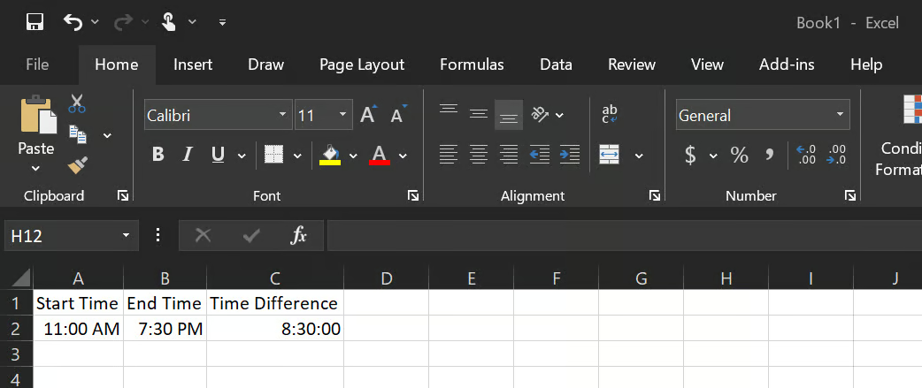
Ora la cella C2 visualizza 8:30:00.

Come puoi notare, è stato usato [h]:mm invece di h:mm perché, senza parentesi, Excel riporta la visualizzazione delle ore a zero dopo le 24. Una durata di 26 ore verrebbe mostrata come 2:00 invece di 26:00. Le parentesi indicano a Excel di mostrare le ore totali, non la lancetta delle ore di un orologio.

Excel supporta sia il formato a 12 ore (AM/PM) sia quello a 24 ore. Una cella che mostra 9:00 AM è equivalente a 09:00, e una che mostra 9:00 PM è equivalente a 21:00. La cosa più importante è usare il formato corretto nelle celle, così i calcoli funzionano come previsto.

Come calcolare il tempo trascorso in Excel

Tempo trascorso e differenza oraria sono due concetti simili ma distinti. 

Mentre la differenza oraria, come detto prima, calcola l’intervallo tra due orari nella stessa giornata, il tempo trascorso si estende su più giorni e richiede valori completi di data e ora (timestamp) per essere calcolato correttamente.

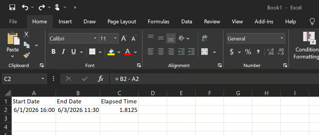
La formula è questa: 

= enddate_timestamp - startdate_timestamp

Entrambe le celle devono contenere una data e un’ora complete. Per esempio, 3/1/2026 14:00 and 3/3/2026 9:30.

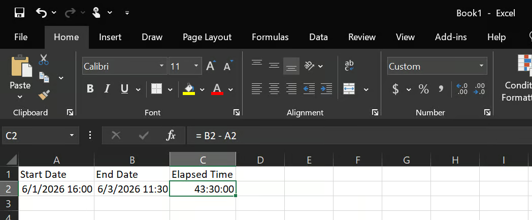
Quando formatti la cella C2 come [h]:mm, il risultato diventa 43:30, che semplicemente significa 43 ore e 30 minuti di tempo trascorso. 

Durante questi calcoli, potresti imbatterti in errori, ad esempio la tua cella che mostra ######## o valori negativi, e più avanti spiegherò come risolverli. 

Come calcolare il tempo tra date in Excel

Per il calcolo della differenza tra date, il concetto è leggermente diverso rispetto a ore e minuti. Excel memorizza le date come numeri seriali (1 gennaio 1900 è 1, 2 gennaio 1900 è 2), quindi puoi sottrarre facilmente le date e trovare l’intervallo.

Per calcolare il numero di giorni tra due date, basta sottrarre la data di inizio dalla data di fine (= end_date - start_date). 

Ecco cosa intendo:

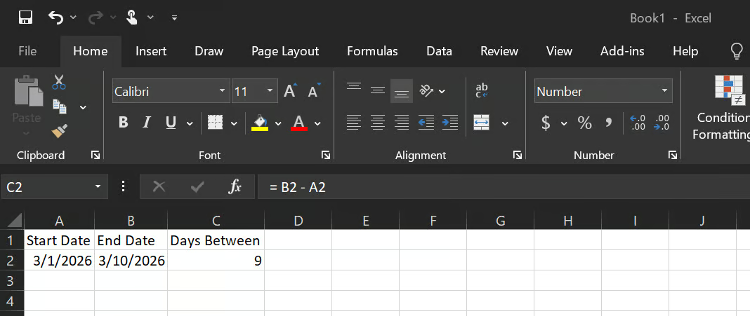
Il risultato sarà 9 giorni, ma assicurati di formattare la cella come numero; in caso contrario, Excel visualizzerà il numero come una data invece che come conteggio dei giorni.

Una volta ottenuto il numero di giorni, puoi convertirlo facilmente per calcolare il numero di ore e minuti, moltiplicando:

• Ore tra date = (End_Date - Start_Date) * 24

• Minuti tra date = (End_Date - Start_Date) * 24 * 60

Guarda questo esempio:

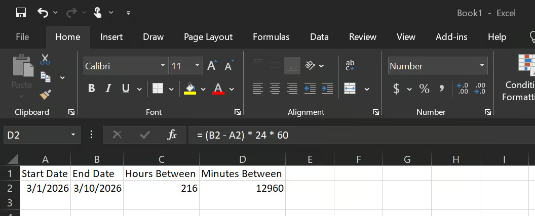
Ore tra date (numero di ore tra le due date) = 216 ore

Minuti tra date (numero di minuti tra le due date) = 12.960

In Excel esiste una funzione che consente di calcolare le differenze in unità specifiche (giorni, mesi e anni), chiamata DATEDIF(). Per eseguire questi calcoli, ecco la logica:

= DATEDIF(Start_Date, End_Date, "d")   → Total difference in days

= DATEDIF(Start_Date, End_Date, "m")   → Total difference in months

= DATEDIF(Start_Date, End_Date, "y")   → Total difference in years

Se vuoi capire i concetti di base in Excel, ti consiglio di dare un’occhiata al nostro percorso Excel Fundamentals.

Come calcolare il tempo totale in Excel

La somma di un elenco di voci orarie in Excel funziona esattamente come la somma per altri tipi di dati.

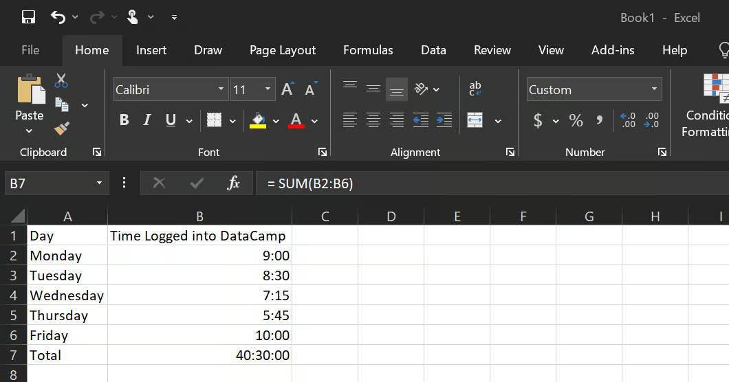
= SUM(C2:C15)

Il problema sorge quando la somma di tutte le voci supera le 24 ore, facendo tornare il conteggio a 0. La soluzione è la stessa che ho descritto dall’inizio: formattare la cella della somma come [h]:mm. 

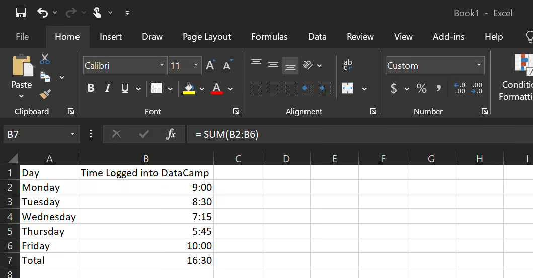
Senza formattare la cella totale (B7), il risultato sarebbe 16:30, ma una volta formattata, il risultato diventa 40:30.

Per gestire in modo efficiente somme orarie elevate, il formato [h]:mm gestisce qualsiasi totale senza limite superiore. Inoltre, per i report, potresti voler convertire il totale in ore decimali:

= SUM(B2:B6) * 24

Questo restituisce 40,0 invece di 40:00, cioè un numero semplice che funziona bene in ulteriori calcoli come moltiplicazioni, divisioni o visualizzazioni.

Come calcolare il tempo medio in Excel

Excel calcola il tempo medio proprio come fa con gli altri numeri usando la funzione AVERAGE(); tuttavia, problemi di formattazione possono impedire di vedere risultati corretti.

La logica da seguire è questa: 

= AVERAGE(B2:B8)

Se la cella del risultato è formattata come "Generale", vedrai qualcosa come 0.354. Applica la formattazione h:mm e verrà visualizzato 8:30. Usa h:mm (senza parentesi) per le medie, perché raramente superano le 24 ore.

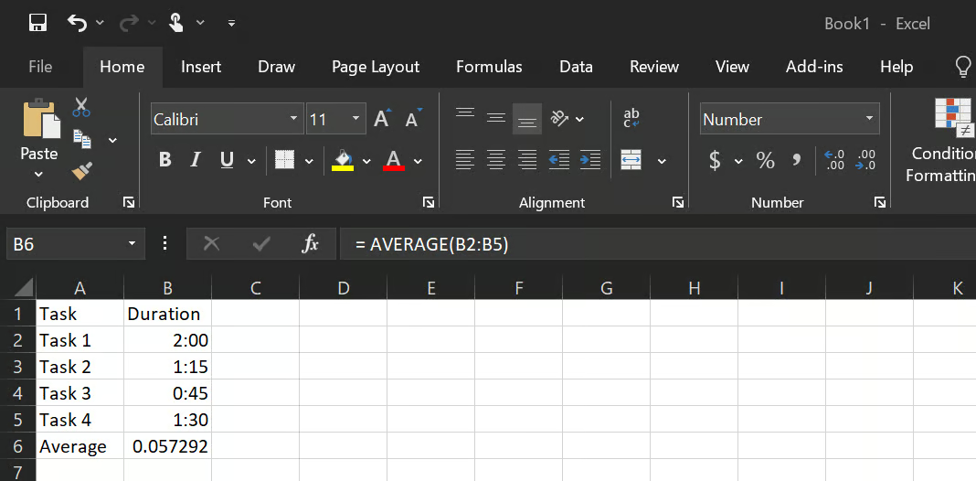
La cella B6 potrebbe inizialmente mostrare 0.057292, ma una volta formattata con h:mm, il risultato diventa 1:22:30 (1 ora, 22 minuti e 30 secondi).

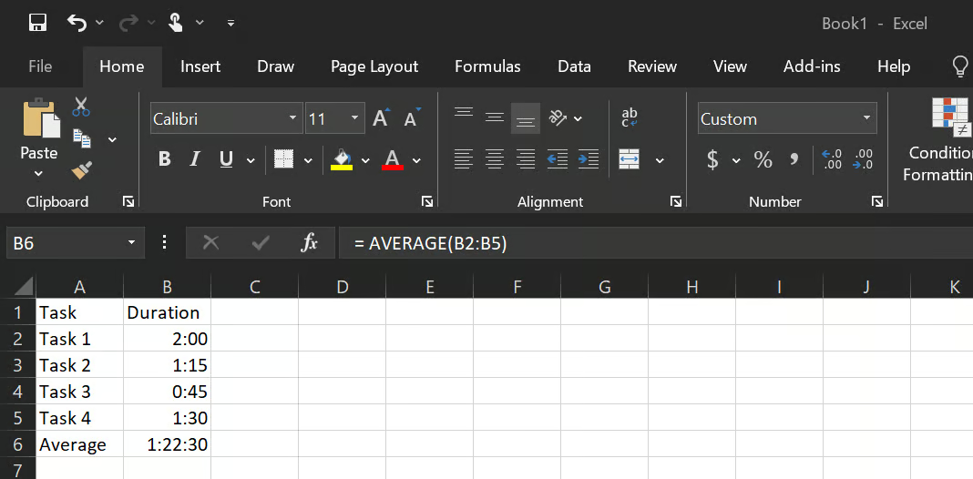
Come spiegato nella sezione sul tempo trascorso, anche in questo caso si applica la stessa formattazione [h]:mm.

Potrebbero anche esserci situazioni in cui i tuoi dataset contengono celle vuote; Excel le ignora automaticamente nel calcolo della media, quindi se hai sette righe di dati con due celle vuote, Excel le considera cinque.

Tuttavia, se la tua cella contiene 0, Excel lo conta e questo può influire sui risultati; in questo caso usa la funzione AVERAGEIF(), utile anche per medie condizionali (quando vuoi la media di righe maggiori, minori o uguali a un certo valore).

= AVERAGEIF(A2:A10, “>0”)

Errori comuni nel calcolo del tempo in Excel

Ci sono alcuni errori comuni in cui potresti imbatterti quando calcoli il tempo in Excel. Ecco quali sono e come risolverli quando capitano:

Valori temporali negativi o ####### 

######## significa che la colonna è troppo stretta per mostrare il risultato; allargala e si risolve. Un valore negativo, invece, di solito significa che le celle di inizio e fine sono state scambiate o che mancano le date in un calcolo che attraversa la mezzanotte. 

Puoi correggere così:

= IF(B2 < A2, B2 + 1 - A2, B2 - A2)

Funziona così: se l’ora di inizio è 18:00 e l’ora di fine è 2:00, B2 < A2 verifica se l’ora di fine è minore di quella di inizio e, se vero, aggiunge un giorno intero (1); altrimenti, sottrae normalmente.

Formattazione errata 

Se il totale sembra più piccolo del previsto o non ti sembra accurato, risolvi usando la formattazione corretta ([h]:mm) come detto in precedenza.

Testo vs valori orari 

Se inserisci un’ora come testo (di solito allineata a sinistra nella cella o digitata con un apostrofo iniziale), qualsiasi calcolo fallisce. Puoi convertire il testo in un valore orario reale usando: = TIMEVALUE(A2) e poi formattare la cella come h:mm.

Confusione per il riavvolgimento a 24 ore 

Quando una SUM() mostra un numero piccolo, è più un problema di formattazione che di formula. Applica [h]:mm alla cella del totale e si sistema.

Buone pratiche per i calcoli del tempo in Excel

Alcune buone pratiche che ti consiglio sono:

• Controlla il formato della cella prima di dare per scontato che una formula sia sbagliata. La maggior parte dei risultati “sballati” sul tempo sono problemi di visualizzazione, non di calcolo.

• Usa [h]:mm per qualsiasi cella che calcola una somma o un totale. Usa h:mm per singole voci orarie all’interno della stessa giornata.

• Non inserire mai orari come testo. Digita 8:30 e lascia che Excel lo riconosca automaticamente. Evita apostrofi iniziali o etichette testuali mescolate ai dati orari.

• Includi le date in qualsiasi calcolo che attraversa la mezzanotte. Un valore solo orario non ha il concetto del giorno successivo.

• Converti in ore decimali prima di usare il tempo in formule finanziarie o di tariffa. Moltiplica il valore orario per 24 per ottenere un numero semplice, poi usalo in moltiplicazioni o divisioni.

• Mantieni formati orari coerenti in tutto il foglio. Una colonna che mescola notazione AM/PM e a 24 ore è un problema di debug futuro.

Conclusione

Calcolare il tempo in Excel non è complicato una volta capito che è solo una frazione di una giornata. 

Gli scenari che abbiamo trattato – differenza oraria, tempo trascorso, intervalli su più giorni, totali settimanali, medie – si riducono alle stesse operazioni di base: sottrazione, addizione e formattazione. La formattazione è il passaggio che molte guide sorvolano, ed è la fonte della maggior parte della confusione.

Se vuoi andare oltre con Excel, il nostro percorso Excel Fundamentals è un itinerario ben strutturato che tocca funzioni, tipi di dati e lavoro con i dataset in Excel.