Kernel trick explicado: como SVMs aprendem padrões não lineares

Modelos lineares são simples e intuitivos, mas falham assim que seus dados não são linearmente separáveis.

E a maioria dos dados do mundo real não é. Por mais que você ajuste os pesos, uma fronteira de decisão reta não resolve — as classes se sobrepõem ou formam padrões que nenhuma linha consegue separar sem erros. Se você sabe que o modelo é simples demais para a tarefa, mas não quer pular direto para uma rede neural, existe um meio-termo inteligente.

Support Vector Machines trazem um “truque”. Você pode projetar seus dados em um espaço de maior dimensão e, o que parecia inseparável, muitas vezes passa a ser separável. O kernel trick é um atalho computacional que permite que modelos baseados em kernel, como SVMs, operem como se os dados tivessem sido transformados — sem nunca realizar essa transformação explicitamente.

Neste artigo, você vai entender exatamente como o kernel trick funciona dentro de SVMs, quais funções kernel valem conhecer e quando os métodos de kernel valem a pena.

Mas o que é SVM, afinal? Leia nosso post sobre Support Vector Machines com Scikit-learn para conhecer o algoritmo e como aplicá-lo.

O que é o kernel trick?

O kernel trick é um método para calcular produtos internos em um espaço de features de maior dimensão sem mapear os dados explicitamente para lá.

Ou seja, você não está realmente transformando seus pontos de dados para depois fazer contas neles. Você calcula qual seria o resultado dessas contas usando uma função kernel que opera diretamente nas entradas originais.

Vale lembrar que o kernel trick só se aplica a modelos que dependem de produtos escalares entre pontos de dados. Não é uma técnica de ML para todos os casos. Se um modelo não usa produtos escalares internamente, o kernel trick não se aplica. A maioria dos modelos não usa.

SVMs, processos gaussianos e kernel PCA são bons exemplos em que esse truque funciona. Mas não deixe ninguém te dizer que isso é algo que “a maioria dos modelos de ML usa”.

Por que o kernel trick existe

Modelos lineares só aprendem fronteiras de decisão lineares. Essa é a restrição rígida deles, e é o que os torna fáceis de entender e interpretar.

Mas a maior parte dos conjuntos de dados reais não é linearmente separável. Não existe uma linha reta (ou hiperplano) que separe as classes de forma limpa. Com o kernel trick, ao projetar esses dados em um espaço de maior dimensão, os mesmos dados podem se tornar separáveis.

A forma óbvia de atacar o problema é transformar os dados explicitamente criando novas features, mapeando cada ponto para o espaço de maior dimensão e treinando o modelo a partir daí. Funciona, mas o custo cresce junto. Se você está mapeando para um espaço com milhares de dimensões, armazenar e calcular nesses vetores transformados fica caro.

Com o kernel trick, em vez de calcular a transformação completa φ(x) para cada ponto, você calcula K(x, x′) — uma função kernel que te dá diretamente o mesmo resultado de produto interno.

O kernel trick em Support Vector Machines

Uma SVM encontra a fronteira de decisão que maximiza a margem entre duas classes.

Para encontrar essa fronteira, a SVM resolve um problema de otimização. E, na sua forma dual, a otimização depende apenas de produtos escalares entre pontos de dados, não dos pontos em si. A função objetivo dual é assim:

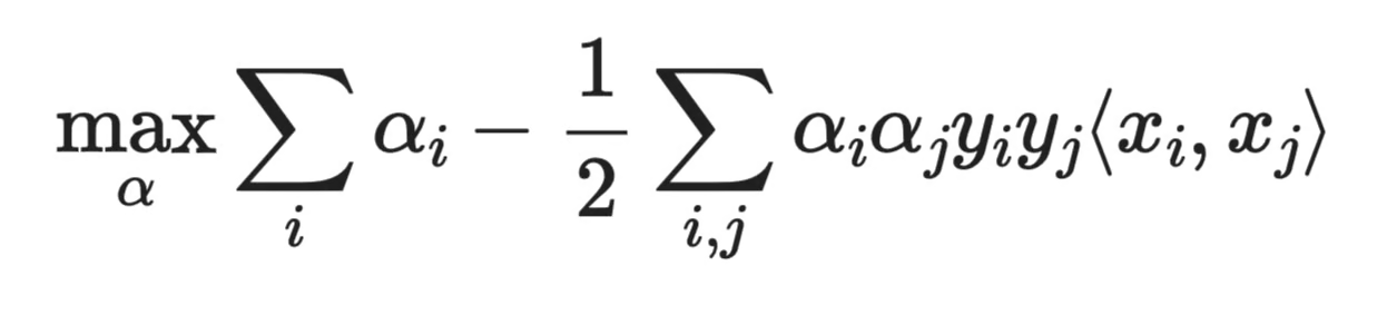
Função objetivo dual

Onde α_i são os pesos aprendidos, y_i são os rótulos de classe, e ⟨x_i, x_j⟩ é o produto escalar entre dois pontos. A SVM só precisa das similaridades par-a-par entre os pontos.

Se a SVM só precisa de produtos escalares, você não precisa fornecer os calculados no espaço original. Basta trocar ⟨x_i, x_j⟩ por uma função kernel K(x_i, x_j):

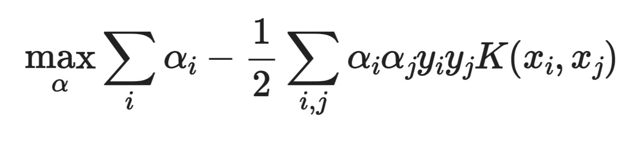
Fórmula com função kernel

A SVM roda exatamente do mesmo jeito. Ela só “pensa” que está operando em um espaço de features mais rico.

E é disso que o kernel trick se trata.

Como o kernel trick funciona (visão conceitual)

A abordagem padrão seria definir um mapeamento φ(x) que transforma cada ponto em um espaço de maior dimensão e, então, calcular produtos escalares lá:

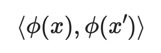
O mapeamento

Mas calcular φ(x) explicitamente pode ser caro e, em alguns casos, o espaço mapeado tem milhares ou até infinitas dimensões.

O kernel trick pula essa etapa.

Em vez de calcular φ(x) e depois fazer o produto escalar, você calcula diretamente K(x, x′) — uma função kernel que satisfaz:

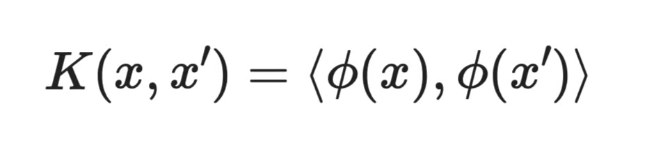
Cálculo com função kernel

O resultado é idêntico, mas o custo é menor.

Pense em K(x, x′) como uma função de similaridade. Ela recebe dois pontos no espaço original e retorna um número que reflete o quão similares eles são — mas de um jeito que corresponde a compará-los em um espaço muito mais rico. O modelo se comporta como se os dados tivessem sido transformados. Eles só não foram.

Funções kernel comuns

Nem toda função kernel funciona da mesma forma. Cada uma define uma noção diferente de similaridade entre pontos, o que significa que cada uma induz um tipo diferente de fronteira de decisão. Veja algumas:

Kernel linear

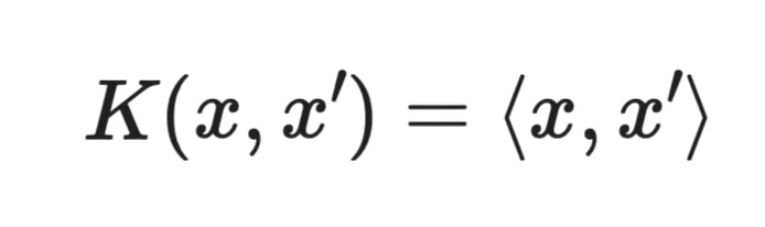
Kernel linear

O kernel linear é apenas o produto escalar padrão. O modelo permanece no espaço de features original e aprende uma fronteira linear, tornando-o equivalente a uma SVM linear tradicional.

Use esse kernel quando seus dados já forem linearmente separáveis. É a opção mais rápida e a mais fácil de interpretar.

Kernel polinomial

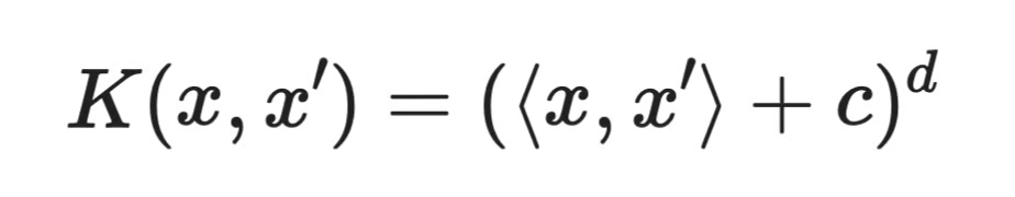
Kernel polinomial

Onde c é uma constante e d é o grau do polinômio.

O kernel polinomial captura interações entre features. Um kernel de grau 2, por exemplo, considera todas as combinações de features em pares. Isso permite que o modelo aprenda fronteiras curvas sem que você precise criar manualmente esses termos de interação.

Graus mais altos significam fronteiras mais expressivas, mas também maior risco de overfitting.

Kernel RBF (Gaussiano)

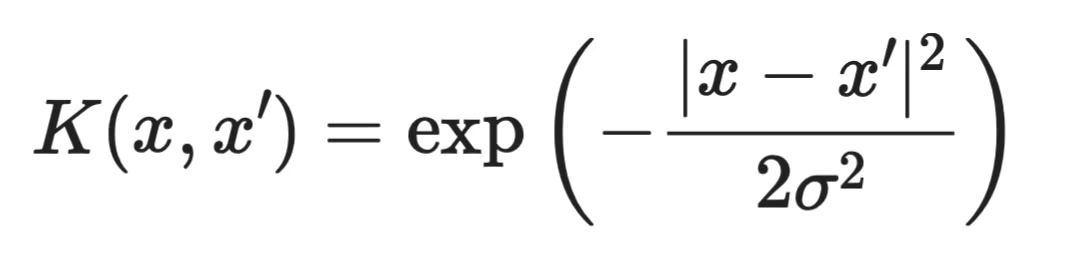
Kernel RBF

O kernel RBF (Radial Basis Function) é o mais usado na prática. Ele mede similaridade com base na distância: dois pontos próximos recebem uma pontuação alta; dois pontos distantes recebem uma pontuação próxima de zero.

O que o torna interessante é que ele mapeia implicitamente os dados para um espaço de dimensão infinita. Isso dá flexibilidade suficiente para capturar fronteiras complexas e não lineares que outros kernels não conseguem.

Kernel sigmoide

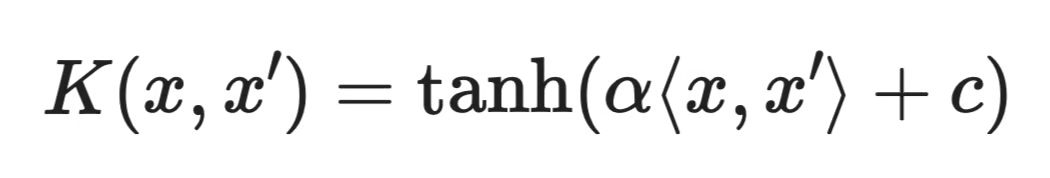
Kernel sigmoide

O kernel sigmoide é menos usado do que os kernels RBF ou polinomial e nem sempre satisfaz as condições matemáticas para ser um kernel válido, dependendo dos parâmetros escolhidos.

Ele aparece ocasionalmente em literatura mais antiga, mas, na prática, RBF quase sempre é um ponto de partida melhor.

Kernel trick além de SVM

SVM é o algoritmo mais comum para aplicar o kernel trick, mas não é o único.

Alguns outros modelos usam a mesma ideia:

• Kernel ridge regression aplica ridge regression em um espaço de maior dimensão usando uma função kernel em vez de features explícitas
• Processos gaussianos usam funções kernel para definir a covariância entre pontos. O kernel codifica suposições sobre a suavidade e o formato da função que você está tentando aprender
• Kernel PCA estende o PCA padrão para estruturas não lineares ao encontrar componentes principais em um espaço de features transformado

Em todos eles, o modelo só precisa de produtos escalares, então você pode trocar por uma função kernel e obter comportamento não linear sem mudar o restante da matemática.

Mesmo assim, SVM segue sendo o exemplo mais claro — e o melhor ponto para construir sua intuição.

Kernel trick vs. engenharia de features

As duas abordagens resolvem o problema de suas features não serem expressivas o suficiente, mas fazem isso de maneiras diferentes.

Com engenharia de features, você cria novas features explicitamente a partir das existentes. Decide quais combinações importam, calcula, adiciona ao seu dataset e treina no conjunto expandido. Você vê exatamente o que entrou no modelo.

O kernel trick opera implicitamente em um espaço de maior dimensão sem que você defina ou armazene essas features extras. A transformação é descrita pela função kernel.

O trade-off está entre interpretabilidade e flexibilidade.

A engenharia de features mantém tudo transparente, pois você sabe o que cada feature representa. O kernel trick te dá mais capacidade expressiva, mas o espaço de features implícito costuma ser difícil de inspecionar ou explicar.

Se interpretabilidade é crucial no seu caso de uso, engenharia de features é a opção mais segura. Se você precisa capturar padrões complexos e não precisa explicar cada decisão do modelo, o kernel trick te leva lá mais rápido.

Vantagens do kernel trick

A mais óbvia é permitir que modelos lineares aprendam fronteiras não lineares. Sem ele, uma SVM só separa classes com um hiperplano reto. Com ele, o mesmo modelo lida com fronteiras curvas e complexas.

Ele também evita o custo de computação explícita em alta dimensão. Você obtém o poder expressivo de um espaço de features mais rico sem armazenar ou calcular aquelas dimensões extras. Para problemas em que o espaço implícito tem milhares ou infinitas dimensões, é isso que torna a abordagem viável.

Métodos de kernel também costumam funcionar bem com datasets de tamanho médio. Quando você não tem milhões de exemplos e seus dados não são linearmente separáveis, uma SVM com um bom kernel costuma ser uma escolha sólida e confiável.

Limitações do kernel trick

O maior problema é a escala. Treinar uma SVM com kernel exige calcular K(x_i, x_j) para cada par de pontos do conjunto de treino. Isso é uma operação O(n²) — e fica ainda pior quando você considera a memória. Em datasets grandes, isso vira um gargalo pesado.

A escolha do kernel também não é trivial. RBF é um bom padrão, mas nem sempre o melhor. Escolher o kernel errado — ou hiperparâmetros ruins — pode acabar entregando desempenho pior do que você tinha.

Interpretabilidade é outro ponto. Com engenharia de features, você sabe o que cada feature significa. Com o kernel trick, o espaço implícito não é claro. O modelo funciona, mas explicar por que ele tomou uma decisão específica é difícil.

E, em muitos domínios, deep learning simplesmente tomou a dianteira. Redes neurais lidam com grandes volumes de dados, aprendem suas próprias representações de features e, muitas vezes, superam métodos de kernel sem exigir seleção manual de kernel. Para classificação de imagens, NLP ou qualquer tarefa com dados massivos, métodos de kernel raramente são a primeira escolha hoje.

Quando usar métodos de kernel

Métodos de kernel não estão obsoletos em 2026, mas ficaram mais especializados do que eram.

Vale apostar em um método de kernel, como uma SVM com kernel RBF, quando:

• Seus dados têm estrutura não linear que um modelo linear não captura
• Seu dataset é pequeno a médio — pense em milhares de amostras, não milhões
• Você não precisa explicar previsões individuais, então menor interpretabilidade é um trade-off aceitável

Eles se encaixam bem em problemas com dados estruturados e tabulares, quando você tem dados limitados e precisa de um modelo que generalize bem sem muito ajuste. Nesses casos, uma SVM com kernel ainda pode superar modelos mais complexos.

Mas, se seu dataset é grande ou você precisa de previsões explicáveis, métodos de kernel não são a melhor solução.

Exemplo: SVM com e sem kernel

A melhor forma de ver o que o kernel trick faz na prática é observar uma SVM linear falhar e, depois, corrigi-la com um kernel.

No exemplo abaixo, temos um dataset simples com dois círculos concêntricos, em que uma classe forma um anel interno e a outra, um anel externo. Não há linha reta que consiga separá-los. Uma SVM linear vai falhar sempre.

Com um kernel RBF, a mesma SVM desenha uma fronteira circular que separa as classes. A única coisa que mudou foi a função kernel.

Aqui vai o exemplo completo:

import numpy as np
import matplotlib.pyplot as plt
from sklearn.svm import SVC
from sklearn.datasets import make_circles

# Generate concentric circles dataset
np.random.seed(42)
X, y = make_circles(n_samples=300, noise=0.1, factor=0.4)

# Train both SVMs
svm_linear = SVC(kernel="linear", C=1)
svm_rbf = SVC(kernel="rbf", C=1, gamma="scale")
svm_linear.fit(X, y)
svm_rbf.fit(X, y)

print(f"Linear SVM accuracy: {svm_linear.score(X, y):.0%}")
print(f"RBF SVM accuracy:    {svm_rbf.score(X, y):.0%}")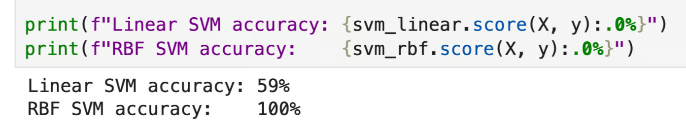

Acurácia: SVM linear vs. RBF

A SVM linear desenha uma fronteira reta no meio dos dados. Ela divide o plano em duas metades, o que não corresponde ao formato real do problema. Já o kernel RBF produz uma fronteira circular que acompanha o desenho dos dados.

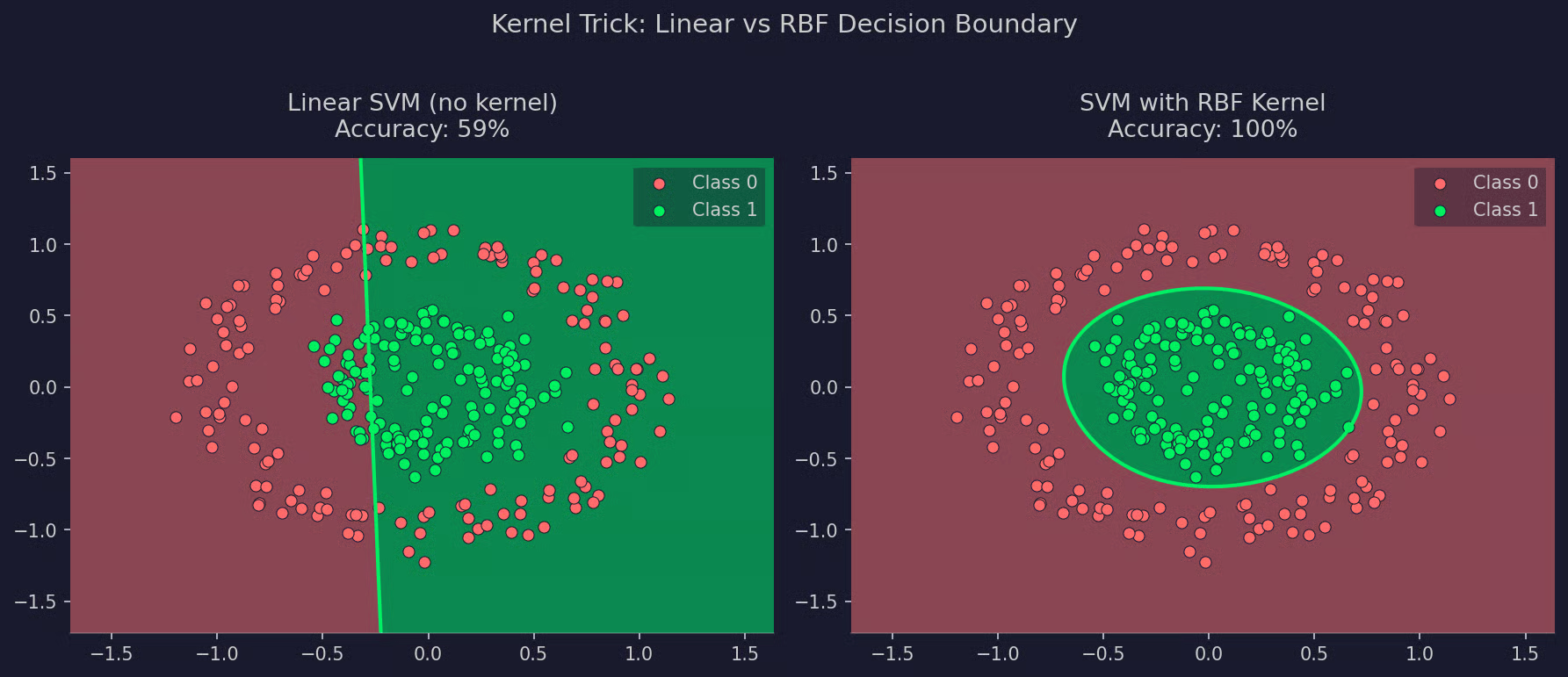
Visualização: SVM linear vs. RBF

Em resumo, o modelo não “aprendeu” uma estrutura mais complexa — ele apenas operou em um espaço onde a estrutura ficou mais fácil de encontrar.

Equívocos comuns sobre o kernel trick

Existem alguns equívocos sobre o kernel trick que aparecem com frequência, então vamos esclarecê-los:

"O kernel trick funciona para todos os modelos." Não funciona. Ele só se aplica a modelos que dependem de produtos escalares entre pontos em sua otimização. A maioria — árvores de decisão, random forests, redes neurais, regressão linear — não usa produtos escalares desse jeito, então o kernel trick não se aplica.

"Ele literalmente transforma os dados." Não de forma explícita. Seus pontos originais continuam iguais. A função kernel calcula o que o produto escalar seria em um espaço de maior dimensão, mas nenhuma transformação acontece na prática. Os dados não são expandidos nem armazenados de outra forma.

"Ele sempre melhora o desempenho." Depende. Em problemas não lineares com datasets pequenos a médios, um bom kernel pode fazer diferença. Em datasets grandes, o custo computacional costuma superar o benefício. E, se seus dados já são linearmente separáveis, adicionar um kernel só adiciona complexidade.

Por que o kernel trick ainda importa

O kernel trick não é o assunto mais falado em ML hoje. Deep learning lidera a maioria dos benchmarks, e métodos de kernel quase não aparecem.

Mesmo assim, é um conceito fundamental que vale entender.

SVMs e o kernel trick foram centrais no ML clássico porque funcionam bem com dados estruturados e tabulares, com poucas amostras, e sua matemática é limpa e bem compreendida. Se você quer entender como o aprendizado baseado em similaridade funciona, ou por que produtos escalares importam em otimização, o kernel trick é um dos exemplos mais claros para estudar.

Ele também ainda tem usos reais. Datasets pequenos, domínios especializados como bioinformática ou classificação de texto com features manuais, e problemas em que você precisa de um modelo que generalize bem com poucos dados — essas são áreas em que métodos de kernel seguem relevantes.

O kernel foi substituído nos domínios em que escala e volume bruto de dados importam mais. No contexto certo, ainda é uma ótima ferramenta.

Conclusão

O kernel trick resolve um problema específico: como extrair comportamento não linear de um modelo que só sabe trabalhar com produtos escalares. A resposta é substituir esses produtos por uma função kernel que computa o mesmo resultado em um espaço de features mais rico — sem realmente ir até lá.

Ele é mais fácil de entender no contexto de SVMs, onde a formulação dual torna a substituição limpa e explícita. Depois que você se acostuma com isso, toda a família de métodos de kernel começa a fazer muito mais sentido.

Deep learning recebe a maior parte da atenção hoje — e, para problemas em grande escala, com razão. Mas o kernel trick representa uma forma diferente de pensar — baseada em geometria e similaridade. Vale entender, embora, a menos que você atue em um nicho específico, dificilmente vá usá-lo com frequência na prática.

Mas por que exatamente o deep learning ganhou espaço? Inscreva-se na nossa trilha Deep Learning in Python para ver como redes neurais permitem construir modelos complexos em escala.