How to Create an Amortization Schedule in Excel: The Steps Explained

An amortization schedule provides a clear financial roadmap, showing how each loan payment splits between interest and principal until your debt is fully paid off.

With Excel's built-in functions, you can create detailed amortization schedules to visualize your loan's lifecycle, make informed financial decisions, and even explore options for early payoff.

In this article, you'll learn how to build a comprehensive amortization schedule in Excel from scratch. We'll cover essential functions like PMT(), IPMT(), and PPMT(), guide you through the step-by-step process, and explore practical scenarios to enhance your financial planning toolkit.

What Exactly Is an Amortization Schedule?

An amortization schedule is a complete table of periodic loan payments, showing the amount of principal and interest that comprise each payment until the loan is paid off at the end of its term.

When you take out a loan, several key elements determine how your payments work:

• Principal: The original amount borrowed that you must repay
• Interest: The cost of borrowing the money, calculated as a percentage of the principal
• Payment period: How often you make payments (monthly, bi-weekly, etc.)
• Loan term: The total time period over which you'll repay the loan

For most standard loans—like mortgages, auto loans, and personal loans—payments remain consistent throughout the term. However, what changes with each payment is the proportion that goes toward interest versus principal. In the early stages, a larger percentage of each payment covers interest. As you progress through the loan term, more of each payment reduces the principal balance.

The primary purpose of creating an amortization schedule is to provide transparency into your loan. It lets you see exactly how much interest you'll pay over time, how quickly you're building equity, and how additional payments might affect your loan timeline. For businesses, these schedules also serve accounting and tax planning purposes.

The Excel Functions and Formulas You Need to Know

Excel does not have a single built-in "amortization" function. Instead, you typically build out an amortization schedule with specific financial functions that work together to calculate different aspects of your loan payments. Here are the key functions you'll need:

PMT() function

The PMT() function calculates the payment for a loan based on constant payments and a constant interest rate:

=PMT(rate, nper, pv, [fv], [type])

• rate: The interest rate per period (annual rate divided by payment frequency)

• nper: The total number of payment periods

• pv: The present value (loan amount)

• [fv]: Optional future value (typically 0 for loans paid in full)

• [type]: Optional; 0 for end-of-period payments, 1 for beginning-of-period

To calculate a monthly payment on a $250,000 mortgage at 4.5% annual interest for 30 years: 

=PMT(4.5%/12, 30*12, 250000)

This returns -$1,266.71, representing the cash outflow for the borrower.

For a detailed explanation of the PMT() function, including common errors and advanced usage examples, you can refer to our comprehensive PMT() Excel guide.

IPMT() function

The IPMT() function calculates the interest portion of a specific payment:

=IPMT(rate, per, nper, pv, [fv], [type])

• per: The specific payment period you're calculating

The per parameter is essential as it determines which payment period's interest amount you're calculating - unlike the PMT() function which gives the same payment amount for all periods, IPMT() results vary significantly depending on which period you specify since interest portions decrease over the loan term.

This shows exactly how much of a given payment goes toward interest.

PPMT() function

The PPMT() function calculates the principal portion of a specific payment:

=PPMT(rate, per, nper, pv, [fv], [type])

Similar to IPMT(), the principal amount varies by period, with earlier payments having smaller principal portions and later payments having larger ones. This shows how much of a given payment reduces your loan balance.

Custom formulas

For each payment period, you'll want to track:

Remaining balance: The outstanding loan amount after each payment

Remaining balance = Previous balance - Current principal payment

Cumulative principal: Total principal paid to date

Cumulative principal = Previous cumulative principal + current principal payment

Cumulative interest: Total interest paid to date

Formula: Previous cumulative interest + current interest payment

Round() function

Even small rounding errors can compound over time in an amortization schedule:

=ROUND(value, 2)

This ensures all monetary values are rounded to the nearest cent.

Absolute vs. relative references

When building your amortization table, you'll need to:

• Use absolute references ($) for fixed values like interest rate and loan amount

• Use relative references for values that change each period

The below formula, for example, uses absolute references for the interest rate, loan term, and amount, but a relative reference for the payment period:

=PPMT($B$2/12, A10, $B$3*12, $B$1)

Step-by-Step Guide to Creating the Amortization Schedule

Now that you understand the key functions, let's build an amortization schedule from scratch. This walkthrough will create a complete loan payment table that tracks each payment throughout the life of your loan.

1. Entering loan data

Enter your loan details in the dedicated input cells as shown in the example below:

• Loan amount: $250,000 (cell B1)
• Annual interest rate: 4.5% (cell B2)
• Loan term: 30 years (cell B3)
• Payment frequency: Monthly (cell B4)

Setting up the loan input parameters. Image by Author. 

2. Calculating the monthly payment

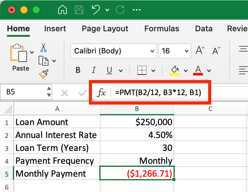
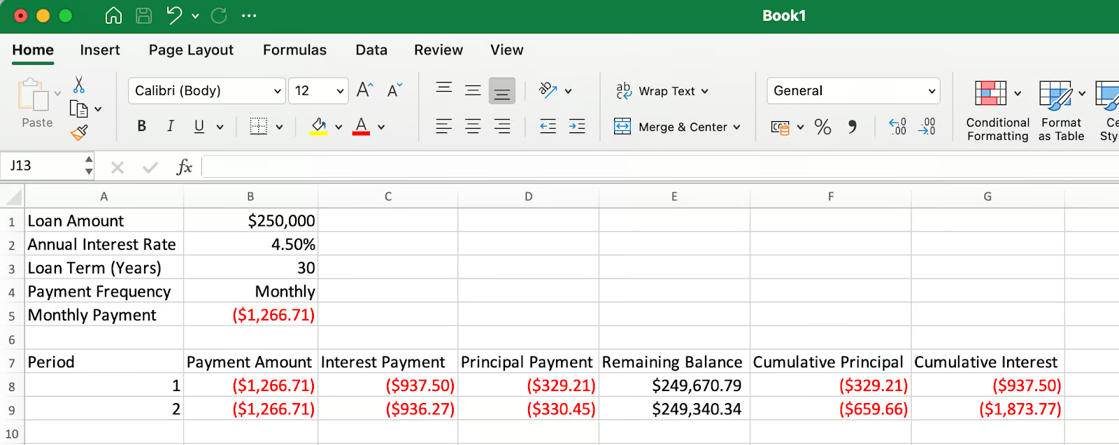
In cell B5, calculate the monthly payment using the PMT function: =PMT(B2/12, B3*12, B1)

This formula returns -$1,266.71, which represents your monthly payment. The negative sign indicates this is a payment (cash outflow).

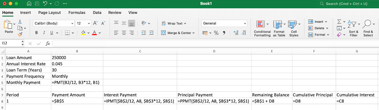
Setting up the column headers and formulas. Image by Author.

3. Creating the first row of the schedule

Next, we can create the following headers and work through the first row of data (rows 7 and 8):  

• Period: Enter 1 in cell A8

• Payment Amount: =$B$5 in cell B8 (referencing the calculated monthly payment)

• Interest Payment: =IPMT($B$2/12, A8, $B$3*12, $B$1) in cell C8

• Principal Payment: =PPMT($B$2/12, A8, $B$3*12, $B$1) in cell D8

• Remaining Balance: =$B$1+D8 in cell E8 (original loan plus principal payment, which works because D8 returns a negative value, effectively subtracting the principal amount from the loan)

• Cumulative Principal: =D8 in cell F8 (same as the principal payment for first row)

• Cumulative Interest: =C8 in cell G8 (same as the interest payment for first row)

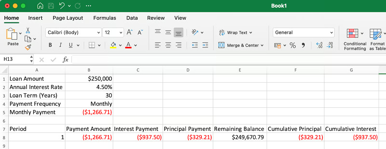
Showing the breakdown of the first payment. Image by Author.

4. Completing the schedule

For the second row (row 9):

• Period: =A8+1 in cell A9 (incrementing by 1)

• Payment Amount: Copy the formula from B8 to B9

• Interest Payment: =IPMT($B$2/12, A9, $B$3*12, $B$1) in cell C9

• Principal Payment: =PPMT($B$2/12, A9, $B$3*12, $B$1) in cell D9

• Remaining Balance: =E8+D9 in cell E9 (previous balance plus current principal)

• Cumulative Principal: =F8+D9 in cell F9 (previous total plus current principal)

• Cumulative Interest: =G8+C9 in cell G9 (previous total plus current interest)

Note that in both the IPMT() and PPMT() functions, A9 is used as a relative reference (without dollar signs), which means when you copy the formula down, it will automatically update to A10, A11, etc., calculating the correct period each time.

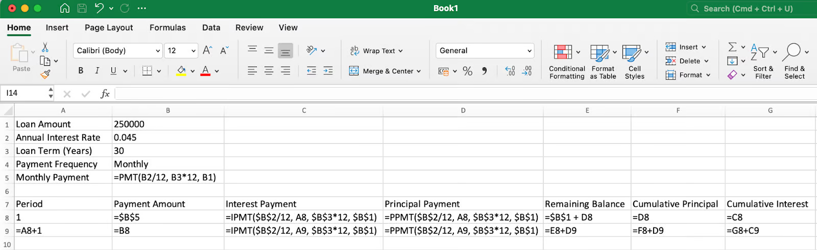
Setting up formulasthat can be copied down . Image by Author.

The first several payments in the amortization schedule. Image by Author.

Select all cells in row 9 and drag down to row 367 (for a 30-year monthly loan with 360 payments).

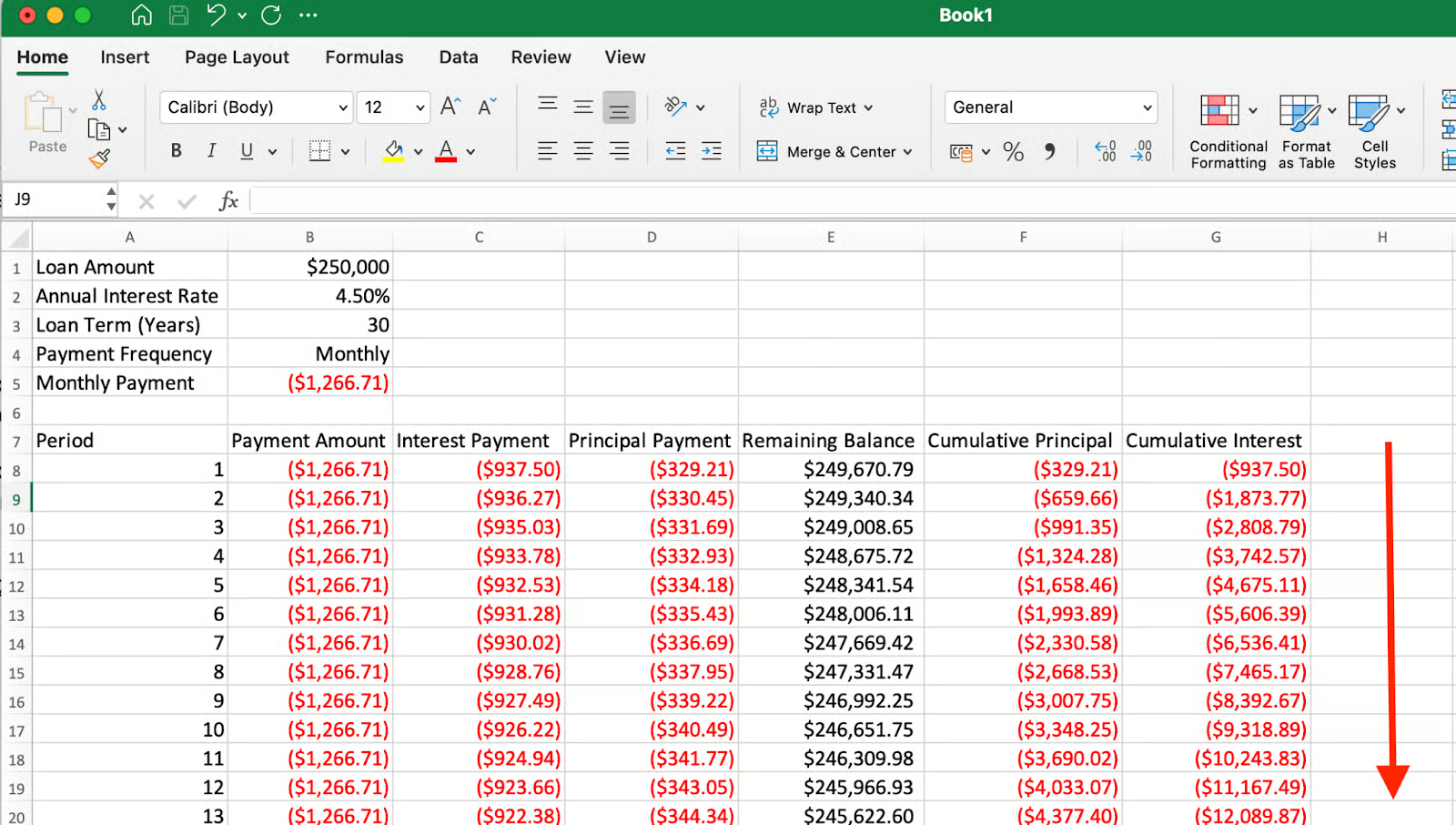
As you progress through the loan term, more of each payment goes toward principal rather than interest. Image by Author.

5. Verifying the final payment

In a properly constructed amortization schedule, the final payment should bring the remaining balance to exactly zero, and the cumulative principal should equal the original loan amount.

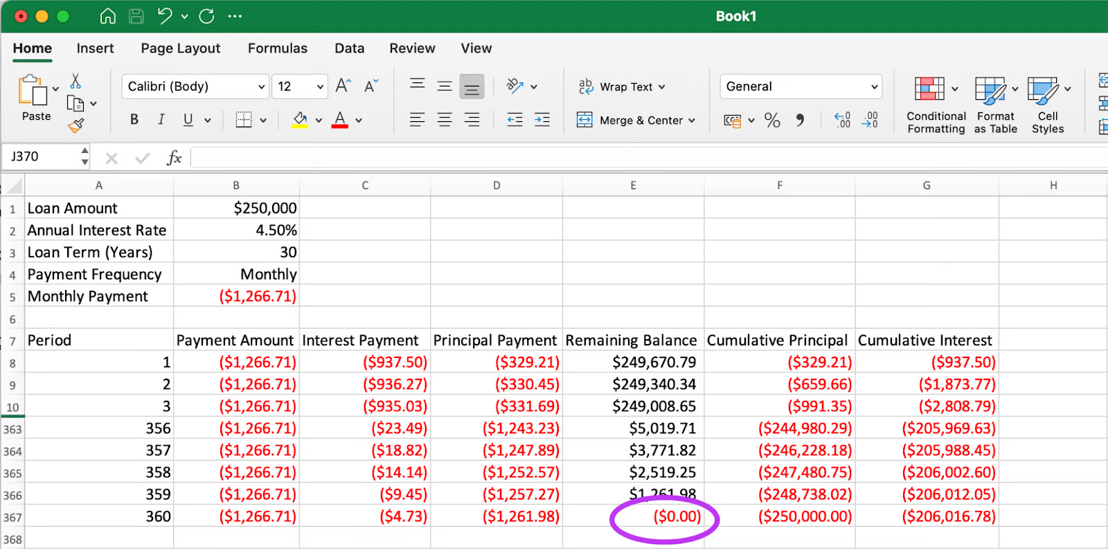
The final payment brings the remaining balance to exactly zero. Image by Author.

As you can see in the final row, the remaining balance is $0.00 (highlighted), and the cumulative principal equals $250,000, which matches our original loan amount. This confirms that our amortization schedule is accurate.

When verifying the final balance, applying the ROUND() function to key calculations can be useful. Small decimal discrepancies due to Excel's calculation precision might cause the final balance to show a tiny residual amount instead of exactly zero. Using =ROUND(value, 2) ensures all monetary values stay consistent with typical financial reporting standards.

Additional Things You Might Want to Consider

A standard schedule is the starting point. Consider these things to make your model more flexible:

Managing payment variations

Amortization schedules become even more valuable when customized to explore different payment scenarios. To model extra payments, create an additional input cell for supplemental payments and modify your principal payment formula to include this amount. This approach helps visualize how additional payments reduce both the loan term and total interest paid. For loans with balloon payments or variable interest rates, consider creating separate sections in your schedule that reflect rate changes at specific points. You can use Excel's Scenario Manager to compare different rate environments and their impact on your total costs.

Enhancing readability and analysis

Proper formatting transforms your amortization schedule from a basic table into an insightful financial tool. Apply currency formatting with consistent decimal places to all monetary values, and use conditional formatting to highlight key milestones—like when you've paid off half the principal or reached specific equity thresholds. It's also important to understand how different interest accrual methods affect your payments. Daily accrual (common in student loans) calculates interest based on a 365-day year, while many mortgages use a monthly accrual method. Documenting which method your schedule uses ensures accuracy when comparing to actual loan statements.

Customizing for specific loan types

Different loans have unique characteristics that may require adjustments to your basic amortization template. For mortgages with escrow accounts, add columns to track insurance and tax components alongside principal and interest. For loans with negative amortization (where payments don't cover accrued interest), modify your remaining balance calculation to add unpaid interest to the principal. The payment timing option in Excel's financial functions (type parameter) lets you model payments at the beginning or end of periods, which is particularly useful for leases and some commercial loans where timing conventions differ from standard consumer loans.

Conclusion

Creating an amortization schedule in Excel gives you valuable insight into your loans beyond what most lenders provide. By building your own schedule, you can see exactly how each payment affects your balance, understand the true cost of borrowing over time, and make informed decisions about prepayment options. The skills developed through this process—using Excel's financial functions, creating dynamic formulas, and designing informative tables—extend far beyond loan analysis and can be applied to many aspects of personal and business financial planning.

If you'd like to go beyond amortization and build more complete financial models—including forecasting income, evaluating investments, and running what-if scenarios—check out our Financial Modeling in Excel course. It's a great next step to strengthen your spreadsheet skills for financial analysis. And remember, the more comfortable you become with these financial calculations, the better positioned you'll be to take control of your financial future, whether you're managing personal debt, planning business investments, or advising clients on their financial options.