Eigendecomposition: A Beginner's Guide to Matrix Factorization

Operations on matrices constitute the core of computations in machine learning, statistical analysis, and scientific computing. For example, many operations in statistics require matrix inversion, diagonalization, and exponentiation. Such operations are computationally expensive, but there are methods to break down a matrix into a smaller set of matrices and thus increase computation efficiency. These operations are generally referred to as matrix factorization, and depending on the nature of the smaller matrices obtained, they have specific names. 

Eigendecomposition is one method of matrix factorization in which eigenvalues and eigenvectors constitute the elements of those matrices. Understanding matrix eigendecomposition provides machine learning and data science engineers with a mathematical foundation to understand methods such as dimension reduction and matrix approximation. After you read this article, take Linear Algebra for Data Science in R course to learn about the very central mathematical topics underpinning data science.

What is Eigendecomposition?

Eigendecomposition is a matrix factorization method in which a square matrix is factored (decomposed) into three multiplicative matrices. Such factorization is called eigendecomposition because the entries of the matrices are eigenvalues and eigenvectors of the original square matrix. Mathematically, a square matrix A can be factored into three matrices such that:

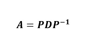
where P is the matrix of the eigenvectors of A, D is a diagonal matrix whose nonzero elements are the ordered eigenvalues of the matrix, and P^-1 is the inverse of the matrix P.

The Mathematics Behind Eigendecomposition

I will demonstrate through an example the mathematical operations to analytically derive the eigendecomposition of a square matrix. Our example matrix is the 2x2 square matrix A. If you get stuck on the techniques for combining matrices, do take our Linear Algebra for Data Science in R course so you feel comfortable with how matrix multiplication works.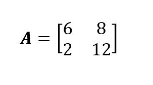

To perform eigendecomposition on matrix A, we need to derive the eigenvalues and the corresponding eigenvectors of this square matrix. We can use the characteristic polynomial of the matrix to compute the eigenvalues and the eigenvectors of this matrix. So if you are unfamiliar with this part, read Characteristic Equation: Everything You Need to Know for Data Science first. 

Now, from the definition of a characteristic polynomial, we have:

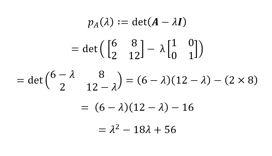
The characteristic polynomial for our matrix A then is p_A(λ) = λ² - 18λ + 56. We can find the roots of this polynomial by equating it to zero to derive the eigenvalues: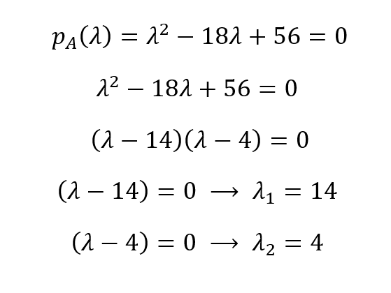 

So, the eigenvalues are λ₁ = 14 and λ₁ = 4. From eigenvalues, we can obtain the eigenvectors of a matrix using (A - λI)X = 0 for each unique eigenvalue: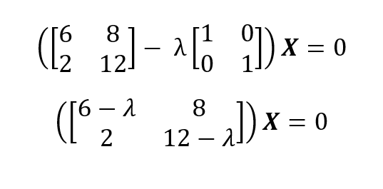

For λ₁ = 14 we plug in 14 and solve the homogeneous system of equations:

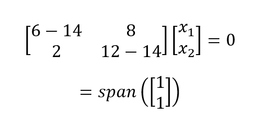
Which gives a one-dimensional (i.e., one basis vector) eigenspace. We perform the same process for λ₁ = 4 and get:

Now that we have obtained the eigenvalues and the eigenvectors of the matrix A, we can write the eigendecomposition of A as:

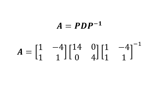
In which we constructed P by collating the two eigenvectors (by which I mean putting them side-by-side) and we placed the eigenvalues (by decreasing order) on the diagonal of the matrix D. 

Of course, we can perform eigendecomposition with a computer system and a programming language like Python or R. Remember that Python and R may produce normalized (on 0-1 scale) eigenvectors (i.e., orthonormal basis). This is important to note when one tries to reconstruct the matrix A from PDP^-1 for verification purposes.

Applications of Eigendecomposition in Data Science

Eigendecomposition plays an important role in machine learning and statistics. In machine learning, eigendecomposition is used for dimension reduction methods, such as PCA. In PCA, we search for new dimensions (directions) for the original high-dimensional coordinates that retain the maximum information. The eigendecomposition of the matrix reveals the eigenvalues, and the eigenvectors with highest eigenvalues retain higher information, and hence are designated as principal components of the data.

Performing Eigendecomposition in Python and R

After having learned how to perform eigendecomposition by pen and paper, we can now perform eigendecomposition using a computer and a programming language, like Python and R in a few lines. Remember that the eigenvectors computed in Python and R are normalized (compared to symbolic programming languages or packages, like SymPy in Python).

Eigendecomposition in Python

To perform eigendecomposition in Python, the module NumPy needs to be installed and imported to the environment. The following code illustrates how to perform eigendecomposition in Python for the square nonsymmetric matrix A:

import numpy as np

A = np.array([[6,8], [2,12]]) 

eigVals, eigVecs = np.linalg.eig(A)

print(eigVals)
print(eigVecs)

[ 4. 14.]
[[-0.9701425  -0.70710678]
 [ 0.24253563 -0.70710678]]

 # Reconstruct the original matrix A
D = np.diag(eigVals)
A_reconstructed = eigVecs @ D @ np.linalg.inv(eigVecs)

print(A_reconstructed)

[[ 6.  8.]
 [ 2. 12.]]

Eigendecomposition in R

Eigendecomposition in R can be performed using the built-in function eigen() and, therefore, there is no need to install and import a package for eigendecomposition of small matrices. The following code in R performs eigendecomposition on matrix A (R sorts the eigenvalues in decreasing order, so the order of eigenvectors is different from that of the Python NumPy output):

A <- matrix(c(6,8,2,12), 2,2, byrow = TRUE)

print(A)

eDecomp <- eigen(A)
eigValues <- eDecomp$values
eigVectors <- eDecomp$vectors

print(eigValues)
print(eigVectors)

[1] 14  4
           [,1]       [,2]
[1,] -0.7071068 -0.9701425
[2,] -0.7071068  0.2425356

A_Reconstructed <- eigVectors %*% diag(eigValues) %*% (solve(eigVectors))

print(A_Reconstructed)

Show in New Window
     [,1] [,2]
[1,]    6    8
[2,]    2   12

Eigendecomposition vs. Singular Value Decomposition (SVD)

Eigendecomposition and singular value decompositions (SVD) are two notable matrix factorization methods that are used in machine learning and scientific computing. Although both of these methods factorize a matrix into three matrices, they have some differences:

• Eigendecomposition is only applicable to square matrices, while SVD can be applied to both square and rectangular matrices.
• In SVD, the resulting matrices include singular scores, while those of eigendecomposition include eigenvalues.
• Because SVD can accommodate nonsquare matrices, it has wider applications than eigendecomposition.

Conclusion

In this brief article on linear algebra, we learned about eigendecomposition, how to perform it by pen and paper, and how to compute it using Python and R. We learned how eigendecomposition is used in machine learning algorithms such as PCA. 

If you strongly interested in becoming a data analyst or data scientist, I strongly recommend taking our Linear Algebra for Data Science in R course so that you have a strong foundation in applied mathematics and programming. Also, enroll in our full Machine Learning Scientist in Python career track to explore supervised, unsupervised, and deep learning.