Excel Substring Techniques: Extract and Format Text

Extracting Text by Position Using Excel Substring Functions

We often want to extract specific parts of a text string, such as a word or sequence of characters, based on their position. Excel provides several built-in functions to help you extract specific portions of text strings. Some of the most common functions are LEFT(), RIGHT(), MID(), TEXTBEFORE(), and TEXTAFTER(). Let’s take a look at each. 

Using the LEFT() Excel substring function

You can use the LEFT() function to extract characters from the beginning of a text string. Here is the syntax:

=LEFT(text, [num_chars])

Here: 

• text refers to the cell address where the original text string is located.

• num_chars refers to the number of characters to be extracted. Its default value is 1.

Let's look at an example. Here, I have some product codes, and I want to extract the first three characters from them. 

=LEFT(A2,3)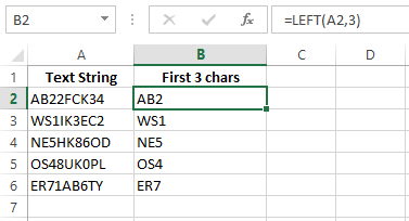

Fetch the first three characters using the LEFT() function. Image by Author.

Using the RIGHT() Excel substring function

The RIGHT() function in Excel extracts characters from the end of a text string. Here is the syntax:

=Right(text, [num_chars])

Here: 

• text refers to the cell address where the original text string is located.

• num_chars refers to the number of characters to be extracted. Its default value is 1.

Let's look at an example. Here, I use the RIGHT() function to extract the last three characters.

=RIGHT(A2, 3)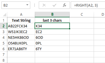

Fetch the last three characters using the RIGHT() function. Image by Author.

Using the MID() Excel substring function

The MID() function extracts characters from the middle of a text string. Here is the syntax:

=MID(text, start_num, num_chars)

Here:

• text refers to the cell address where the original text string is located.

• num_chars refers to the number of characters to be extracted. Its default value is 1.

• start_num refers to the starting position within the text string.

In this example, I use the MID() formula to extract the middle value from the string starting from the fourth character.

=MID(A2,4,3)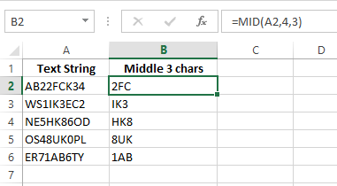

Fetch the mid three characters using the MID() function. Image by Author. 

And it’s done. =MID(A2,4,3) extracts three characters from the text in cell A2, starting from the 4th character.

Using the FIND() Excel substring function

The FIND() function in Excel locates a substring within a text string and returns the position of the first character of the substring within the string. Here is the syntax:

FIND(find_text, within_text, [start_num]) 

Here:

• find_text refers to the text we want to search for.

• within_text is the text containing the text we want to find.

• start_num specifies the position to begin the search, with a default of 1.

Let's consider a simple dataset to show how Excel's FIND() function works. In this example, I have the name DataCamp in the Text column, and I want to locate the position of the substring Camp. This returns 5 because Camp starts at the fifth character in the text.

=FIND("Camp", A2)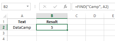

Using the FIND() function to extract the position of the text. Image by Author.

Using the SUBSTITUTE() Excel substring function

The SUBSTITUTE() function replaces a specific substring with another one. Here is the syntax:

 SUBSTITUTE(text, old_text, new_text, [instance_num])

Here:

• text contains the text you want to change.

• old_text refers to the text you want to replace.

• new_text is the text you want to replace the old text with.

• instance_num specifies which occurrence of text you want to change. If not specified, every instance is replaced. 

To understand this, let's look at a simple dataset that contains text strings with specific delimiters. The Text column lists names and ages formatted with semicolons as delimiters. To clean this, I type the following formula:

=SUBSTITUTE(A2, ";" , ",")

Here:

• A2 refers to the cell containing the original text.

• ";" specifies the old text that we are going to change.

• "," is the text we want to replace the old text with.

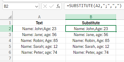
Using the substitute function to replace old text. Image by Author.

And that’s it. By applying our formula in cell B2, Excel replaces the semicolon with a comma.

Extracting Text by Delimiter Using Excel Substring Functions

Delimiters are the specific characters that separate the two text strings, such as a semicolon or a comma. In Excel, you can use the TEXTBEFORE() and TEXTAFTER() functions to extract text when the delimiters are present.  

Using the TEXTBEFORE() Excel substring function 

As the name suggests, the TEXTBEFORE() function extracts text located before a specified character or substring. Its syntax is as follows:

=TEXTBEFORE(text, delimiter, [instance_num], [match_mode], [match_end], [if_not_found]

Here: 

• text refers to the original text.

• delimiter is typically a comma or a semicolon.

• instance_num is the desired occurrence of the delimiter. Its default value is 1.

• match_mode indicates whether the search for the delimiter should be case-sensitive (TRUE, default) or case-insensitive (FALSE).

• match_end determines if the end of the text string should be treated as a delimiter. If TRUE, the function will return the original text if the delimiter isn't found.

• if_not_found specifies a custom value to return if the delimiter isn't found.

Now, let’s take an example to see this formula in action. I have a column Text containing the employee details, including their names, departments, and branch locations. I now want to extract just the names and departments.

=TEXTBEFORE(A2, ",", 2, 1, 1)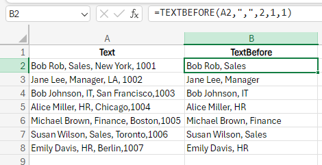

Using TEXTBEFORE() function to extract data. Image by Author 

Here’s how this works: 

• A2 contains the text I want to extract from. 

• "," is the delimiter that splits the text in my original data. 

• 2 means the function will consider the second occurrence of the delimiter.

• 1 ignores case-sensitive instances, if any.

• 1 (in the end) returns the original text if the delimiter is absent.

Using the TEXTAFTER() Excel substring function

The TEXTAFTER() function is similar to the TEXTBEFORE() function—the only difference is in the result. The TEXTAFTER() function extracts text that comes after a delimiter. Its syntax is as follows:

=TEXTAFTER(text, delimiter, [instance_num], [match_mode], [match_end], [if_not_found]

Here: 

• text refers to the original text.

• delimiter is a comma or a semicolon. 

• instance_num is the desired occurrence of the delimiter. Its default value is 1.

• match_mode indicates whether the search for the delimiter should be case-sensitive (TRUE, default) or case-insensitive (FALSE).

• match_end determines if the end of the text string should be treated as a delimiter. If TRUE, the function will return the original text if the delimiter isn't found.

• if_not_found specifies a custom value to return if the delimiter isn't found.

Here, I have a column Text containing the employee details, including their names, departments, and branch locations. From this, I want to extract the employees' locations and IDs. 

=TEXTAFTER(A2,",",2,1,1)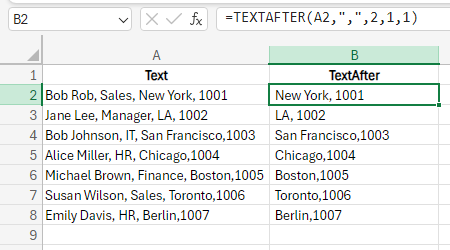

Using the TEXTAFTER() function to extract data. Image by Author 

Here’s how this works: 

• A2 contains the text I want to extract from. 

• ","  is the delimiter that splits the text in my original data. 

• 2 means the function will consider the second occurrence of the delimiter. 

• 1 ignores case-sensitive instances, if any.

• 1 (in the end) returns the original text if the delimiter is absent.

Specific Excel Substring Use Cases

Now that you know the basics of substrings, it’s time to learn the advanced methods. These methods allow more complex text manipulations, making your data processing tasks even more efficient. 

Handling varying lengths of first names

I have a dataset that contains the full name, but I want to extract only the first name.

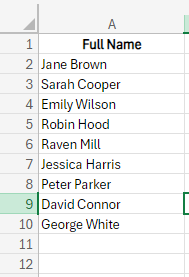
A table containing full names. Image by Author.

You must think it's simple—use the LEFT() function to get the first name. So, I tried it using the formula:

=LEFT(A2,4)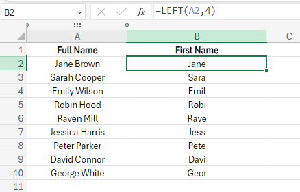

Using the LEFT() function to fetch the first name. Image by Author.

But instead of getting the first name, I got the first four characters from the name because I specified the num_char as 4, seeing that Jane has four characters in the first name. When I copy-paste the formula, it doesn't give the desired output for other names.

I need a more flexible solution. To extract the first name, regardless of the length, you can combine the LEFT() function with the FIND() function. I use the FIND() function to find the position of the first space in the full name, which separates the first and last name. Then, I use the LEFT() function to extract characters up to that position. 

=LEFT(A2,FIND(" ",A2)-1)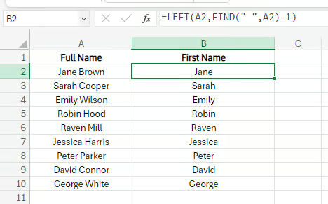

Combine FIND() and LEFT() functions to extract the first name. Image by Author.

Let me break down the formula to help you understand how it works:

• A2 cell contains the full name.

• FIND(" ", A2, 1) finds the position of the first space in the text string in cell A2 starting from the first character.

• -1 is used to remove the space.

• LEFT(A2, ...) extracts the specified number of characters from the left of the text string.

Extracting domain from email address

Let’s take another example to see if  LEFT() and FIND() can handle a different scenario. I have a different dataset of email addresses from which I have to extract the domain name.

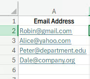
Data containing email addresses. Image by Author.

To do so, I create a different column, Email Domain, and selected a different cell to type the following formula, which I then copy to three other cells:

=RIGHT(A2, LEN(A2) - FIND("@",A2))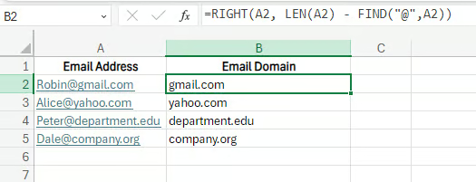

Extract the domain name using RIGHT(), LEN(), and FIND(). Image by Author.

Here you go—I have all the domain names. But let’s understand how Excel retrieves my desired results:

• FIND("@", A2) locates the position of the @ symbol in the email address.

• LEN(A2) calculates the total length of the email address.

• LEN(A2) - FIND("@", A2) computes the number of characters after the @ symbol.

• In the end, RIGHT(A2, LEN(A2) - FIND("@", A2)) extracts that number of characters from the right end of the string.

Extract product codes by combining LEFT(), MID(), and RIGHT()

Until now, I only explained how LEFT(), MID(), and RIGHT() functions work separately. But you can do so much more by combining these functions. They can extract different parts of a text string based on specific patterns.

Here, I have a list of product codes and I want to extract a specific section from them. 

• From the first section, I want one character.
• From the second section, I want all four characters.
• From the last section, I want to extract the last three characters.

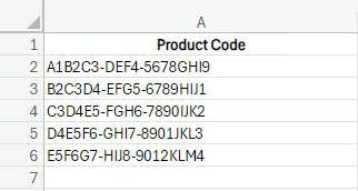
A list of product codes. Image by Author.

To accomplish this, I combine the LEFT(), RIGHT(), and MID() functions and enter the following formula:  

=LEFT(A2, 1) & "-"& MID(A2, FIND("-", A2) + 1, 4) & "-" & RIGHT(A2, 3)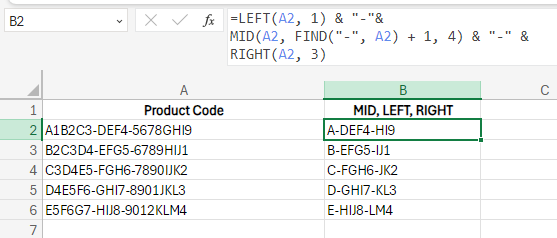

Combine MID(), LEFT(), and RIGHT() functions to fetch data. Image by Author.

As you can see, this combined formula extracted the desired characters from each section from the codes. Here’s how:

• LEFT(A2, 1) extracts the first character.

• MID(A2, FIND("-", A2) + 1, 4) finds the first hyphen, moves one character right, then extracts four characters.

• "-" adds a hyphen.

• RIGHT(A2, 3) extracts the last three characters.

• & concatenates the characters. 

Using SUBSTITUTE() with MID() for dynamic text extraction 

Now, let’s see how you can combine the MID() function with the SUBSTITUTE() function to extract specific portions of a text string and then replace characters or substrings within that extracted part.

For example, I have customer Order Details and want to replace the order ID with the text Order confirmed.

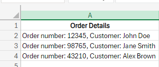
A table containing order details. Image by Author.

I use the following formula:

=SUBSTITUTE(A2, MID(A2,1,19), "Order confirmed")

SUBSTITUTE() and MID() functions to replace the text. Image by Author.

That’s it! You can see this formula extracts specific portions of text strings, as I wanted.

• MID(A2, 1, 19) extracts the first 19 characters from the text in cell A2.

• SUBSTITUTE(text, old_text, new_text) replaces occurrences of old_text with new_text.

Let's look at another example: Here, I have a Product Detail column, and I want to extract the product size from the square bracket.

=SUBSTITUTE(MID(A2, FIND("[", A2)+1, FIND("]", A2)-FIND("[", A2)-1), "[", "")

Extracting the product size from the square bracket. Image by Author.

And it's done—it extracted all the details.

• FIND("[", A2) finds the starting position of the square bracket.

• FIND("]", A2) finds the ending position of the square bracket.

• MID(A2, FIND("[", A2)+1, FIND("]", A2)-FIND("[", A2)-1) extracts the text between the two brackets.

• SUBSTITUTE(...,"[", "") removes the opening square bracket from the extracted text.

Cleaning up data entries

Sometimes, our data is disorganized, but that doesn’t mean you have to use such data in your operations. Here, I have a list of phone numbers in multiple formats, but I want to standardize them in a consistent format by cleaning up any inconsistencies in the entries.

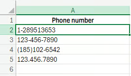
Unformatted phone numbers. Image by Author.

To standardize this, I create a different column called Clean data. I type the following formula in the second cell and I copy this formula to all the cells where I want to see the results:

=SUBSTITUTE(SUBSTITUTE(SUBSTITUTE(SUBSTITUTE(A2, "-", ""), "(", ""), ")", ""), ".", "")

Here: 

• SUBSTITUTE(A2, "-", "") removes hyphens.

• SUBSTITUTE(..., "(", "") removes parentheses.

• SUBSTITUTE(..., ")", "") removes closing parentheses.

• SUBSTITUTE(..., ".", "") removes periods.

This transforms the multiple formats into a continuous string of digits, as shown below. Now, the data is cleaned, nicely formatted, and ready to go. You can leave it as is if you want.

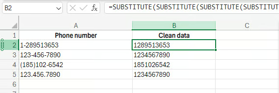
Clean up the data using the SUBSTITUTE() function. Image by Author.

Formatting text for reports

If you want to go the extra mile after data cleaning and format it appropriately, you can also use different substring functions.

Consider the previous example, where I cleaned the phone numbers. Now, I want to change the formatting of the numbers so they look more like phone numbers and not just a string of digits. 

=TEXT(LEFT(B2, 3), "000") & "-" & TEXT(MID(B2, 4, 3), "000") & "-" & TEXT(RIGHT(B2, 4), "0000")

Standardized format of numbers using multiple substrings. Image by Author.

And it's done. I now have all the numbers I wanted. Here’s how this formula worked:

• LEFT(B2, 3) extracts the first three digits.

• MID(B2, 4, 3) extracts the next three digits starting from the fourth position.

• RIGHT(B2, 4) extracts the last four digits.

• TEXT(..., "000") and TEXT(..., "0000") formats each section to ensure the correct number of digits with leading zeros if needed.

• & "-" & joins the formatted sections with hyphens.

Final Thoughts

You've now learned how to use Excel's substring functions like LEFT(), RIGHT(), MID(), TEXTBEFORE(), and TEXTAFTER() to manipulate text data. Whether pulling out specific parts of a string or cleaning up messy data, these functions can make your work much easier and more efficient.

But there's always more to learn with Excel. The Introduction to Excel course is a perfect next step if you're just starting. If you want to learn more about data analysis, try the Data Analysis in Excel course which goes well with our Data Manipulation in Excel Cheat Sheet. These will help you build a strong foundation and take your skills to the next level.