A Beginner’s Guide to Data Cleaning in Python

Introduction to Data Cleaning

When you start a new data project, the data you acquire is rarely perfect for your analysis right off the bat. This makes it essential that you go through the process of cleaning your data at the start of every new project.

Cleaning your data is a process of removing errors, outliers, and inconsistencies and ensuring that all of your data is in a format that is appropriate for your analysis. Data that contains many errors or that hasn’t gone through this data-cleaning process is referred to as dirty data.

This step can feel optional to many junior data professionals, but be assured that it is crucial! Without proper data cleaning, your model can reach the wrong conclusion, your graph can show a fake trend, and your statistics can be wildly inaccurate.

Consider an extremely small dataset. You and your friends are splitting your candy evenly between each of you, and you need to determine how many candies each person gets. You input your data into the table below.

Now if you take the mean of the Number of Candies column, you could come to the conclusion that each person should get 12 candies.

However, if you try to give every person 12 candies, you will run out before everyone gets their share because Sandy was duplicated in your table. There are only 40 candies in your stash instead of 60 (and, in fact, only 4 people, not 5)!

By not taking the time to clean your dataset, you risk your analysis coming to the wrong conclusion.

In the case of splitting candies between friends, the biggest consequence may be a miffed friendship. But in the business world, neglecting to clean your dataset could result in analyses that suggest launching the wrong product, hiring the wrong number of employees, investing in the wrong stock, or even charging a client the wrong price!

Data cleaning is even more important with more complex analyses. With complex analyses, you may not have as firm an expectation of what the results should be, which means you may not recognize when the results are wrong.

A thorough data cleaning, along with careful testing, will help to alleviate these concerns. In this tutorial, we’ll cover what you need to know about the data cleaning process in Python.

Understanding Dirty Data

There are many types of errors and inconsistencies that can contribute to data being dirty. Let’s go over a few of the most common types and why they are problematic.

Missing values

Incomplete data sets are extremely common. Your dataset may be missing several years of data, only have some information on a customer, or not contain your company’s full complement of products.

Missing values can have multiple effects on your analysis. Large portions of crucial data missing can cause bias in your results. Additionally, NaN values or missing cells in a DataFrame may break some Python code, causing a lot of frustration while building your model.

Outliers

Outliers are values that are far outside the norm and not representative of the data. Outliers can be the result of a typo or exceptional circumstances. It is important to differentiate true outliers from informative extreme situations. Outliers can skew your results, ultimately suggesting the wrong answer.

Duplicates

As we saw above, duplicate data entries can overrepresent one entry in your analysis, leading to the wrong conclusion. Be aware of duplicates that occur more than once and those that contain conflicting or updated information.

Erroneous data

Sometimes, the values in our data set are simply wrong. You may have the wrong spelling for a customer’s name, the wrong product number, outdated information, or incorrectly labeled data.

It can sometimes be challenging to determine if your data is erroneous, which is why verification of your source is so important! Remember, your analysis is only as good as your data.

Inconsistencies

Inconsistencies come in many forms. There can be inconsistent data entries, which may point to a typo or an error. If you see a customer age backward, an ingredient that changes ID number, or a product with two simultaneous prices, it is worth a closer look to make sure everything is correct.

Another problematic type of inconsistency is inconsistency in the format of the data. Different values may be reported in different units (kilometers vs. miles vs. inches), in different styles (Month Day, Year vs. Day-Month-Year), in different data types (floats vs. integers), or even in different file types (.jpg vs. .png).

These inconsistencies will make it challenging, if not impossible, for your code to interpret the values correctly. This may result in an incorrect analysis or in your code not running at all.

Data Exploration and Preprocessing

It is crucial that you understand your dataset before you use it in a complex analysis. To develop this kind of understanding of your data, you should do some data exploration. You can think of this step as the pre-analysis analysis.

Let’s look at some typical steps for conducting a data exploration on a table-formatted dataset:

1. First and foremost, look at the source of your dataset and determine if that source has any bias or agenda that may affect the quality or reliability of your data.
2. Learn the context of your data and any other factors that may have affected your data that aren’t internally accounted for.
3. Determine how many different variables you have. In a table-formatted dataset, the variables are typically the columns, while each data entry is a row.
4. Determine how many different categories within each variable you have. For example, if one of your variables is Type of Fruit, you should have a good idea of how many different types of fruit are represented within this variable.
5. Look at the summary statistics for each column, including the mean, median, variance, and standard deviation.
6. If possible, plot each variable and as many pairs of variables as you can and really look at the plots. Look for any skews, outliers, trends, or correlations that may be worth looking into further.
7. If your dataset is part of a relational database, look closely at the relationships and make sure you understand how the different tables relate to each other.
8. If applicable, use the profiling feature of the pandas library to generate a profile report. This will provide you with valuable information about your dataset.

Why exploration and preprocessing matters

This all may seem superfluous to your intended analysis, but there are a few important reasons you should always take these steps. Firstly, doing this will give you a great understanding of the limits of your dataset, which is essential if you are to trust the results of your final analyses.

Secondly, data exploration can point you in the direction of important trends and analyses you hadn’t considered previously. These have the potential to add to your intended analyses or to present a complicating factor that you need to take into account.

Thirdly, this pre-analysis can be your first clue to where you may have dirty data. This can be the first time you see that outlier, realize there are twice as many categories as there should be, or discover that the data collection method was different last year than it was the year before. These are all critical pieces of information that should encourage you to be curious about your dataset.

For more information on data exploration, check out DataCamp’s Data Exploration in Python course or this tutorial for absolute beginners.

Techniques for Data Cleaning in Python

Let’s get into some nitty-gritty with some data cleaning techniques in Python by addressing how to deal with some common dirty data problems.

Handling missing values

Invariably, when you have a large dataset, some fields will be missing in one or more entries. Not only does this mean you are missing valuable data, but the NaN entries can trip up some Python functions, making your model inaccurate.

When you find a missing value, you have a choice to either eliminate that entry from analysis or try to impute a reasonable value to put in its place. If your dataset is reasonably small, I would suggest viewing the rows that contain missing values so you can determine the best course of action.

import pandas as pd
 
# Identify rows with NaN values
rows_with_nan = df[df.isnull().any(axis=1)]
 
#View the rows with NaN values
print(rows_with_nan)

Deleting an entry is typically not the first choice, as it means taking potentially valuable information out of the analysis.

However, sometimes deletion is the best option, for example, if the entry doesn’t provide enough other information to warrant keeping it (like if the entry is only a date with no valuable information).

Deletion is also the easiest way to deal with entries that contain missing values. So, if you are short on time and the rest of the entry is not important to the analysis, deleting entries with NaNs is an option.

You can use the .dropna() method from the Pandas library to drop rows from a DataFrame that contain NaNs.

import pandas as pd
 
# Assuming df is your DataFrame
df.dropna(inplace=True)

The generally preferred method of handling missing values is imputing a reasonable value. Finding a reasonable value to impute can be an art in its own right, but there are several established methods that can be a good starting point.

The .fillna() method from Pandas will impute missing values using the mean so as not to change the distribution.

import pandas as pd
 
# Assuming df is your DataFrame
# Replace NaN values with the mean of the column
df.fillna(df.mean(), inplace=True)

The sci-kit learn library has a simple imputation function that works well, too.

from sklearn.impute import SimpleImputer
import pandas as pd
 
# Assuming df is your DataFrame
imputer = SimpleImputer(strategy='mean')
df_imputed = pd.DataFrame(imputer.fit_transform(df), columns=df.columns)

If you need a more complex imputation method, you may consider using a KNN or regression imputation to find a good value. Ultimately, the method you choose will depend on your data, your needs, and your available resources.

Outlier detection and treatment

Outliers are a bit tricky to deal with. Some seeming outliers are actually important data, such as how the stock market responds to crises like COVID-19 and the Global Recession. However, others may be typos or irrelevant, rare circumstances, and should be removed.

Knowing the difference is often a matter of understanding your data in context, which your previous data exploration should have helped you with, and having a clear idea of your goal for your analysis.

Many outliers are visible when the data is plotted, but you can also use statistical methods to identify outliers.

A common method is to calculate a Z-score for each data point and eliminate the values with an extreme Z-score.

import numpy as np
import pandas as pd
 
# Generate some sample data
np.random.seed(0)
data = np.random.randint(low=0, high=11, size=1000)

# Add some outliers
data[0] = 100
data[1] = -100
 
# Calculate Z-scores
z_scores = (data - np.mean(data)) / np.std(data)
 
# Identify outliers based on Z-score threshold (e.g., 3)
threshold = 3
outliers = np.where(np.abs(z_scores) > threshold)[0]
 
print("Outliers identified using Z-score method:")
print(data[outliers])

Another method is to calculate the interquartile range (IQR) of the distribution and classify any values that are Q1-(1.5 x IQR) or Q3 + (1.5 x IQR) as potential outliers.

import numpy as np
import pandas as pd
 
# Generate some sample data
np.random.seed(0)
data = np.random.randint(low=0, high=11, size=1000)
# Add some outliers
data[0] = 100
data[1] = -100
 
# Calculate quartiles and IQR
q1 = np.percentile(data, 25)
q3 = np.percentile(data, 75)
iqr = q3 - q1
 
# Identify outliers based on IQR
lower_bound = q1 - (1.5 * iqr)
upper_bound = q3 + (1.5 * iqr)
outliers = np.where((data < lower_bound) | (data > upper_bound))[0]
 
print("Outliers identified using IQR method:")
print(data[outliers])

Once you have identified any outliers and determined they are problematic, several methods exist to deal with them. If you have determined that the outlier is due to an error, it may be possible to simply correct the error to resolve the outlier.

In other cases, it may be possible to remove the outlier from the dataset or replace it with a less extreme value that retains the overall shape of the distribution.

Capping is a method where you set a cap, or threshold, on your data’s distribution and replace any values outside those bounds with a specified value.

import pandas as pd
import numpy as np
 
# Create a sample DataFrame with outliers
data = {
    'A': [100, 90, 85, 88, 110, 115, 120, 130, 140],
    'B': [1, 2, 3, 4, 5, 6, 7, 8, 9]
}
df = pd.DataFrame(data)
 
# Define the lower and upper thresholds for capping (Here I used the 5th and 95th percentiles)
lower_threshold = df.quantile(0.05)
upper_threshold = df.quantile(0.95)
 
# Cap outliers
capped_df = df.clip(lower=lower_threshold, upper=upper_threshold, axis=1)
 
print("Original DataFrame:")
print(df)
print("\nCapped DataFrame:")
print(capped_df)

In some cases, you can transform your data in a way that makes outliers less impactful, such as a square root transformation or a logarithmic transformation.

Be cautious when transforming your data, as you may introduce more problems in the long run if you’re not careful. There are a few things to consider before deciding to transform your data.

1. Understand the underlying data distribution: Before applying any transformation, it's important to understand the distribution of your data and how certain transformations will impact it.
2. Choose an appropriate transformation: Select a transformation method that is suitable for your data distribution.
3. Handle zeros and negative values: Some transformations may not be suitable for data containing zeros or negative values. Adding a small constant can help avoid issues when taking logarithms, for example.
4. Validate transformed data: After applying transformations, validate the transformed data to ensure that the resulting distribution meets the assumptions of your analysis.
5. Consider the interpretability: Transformed data may not be as easily interpretable as the original data. Ensure that stakeholders understand the implications of the transformation on the interpretation of results.

To learn more about data transformations, I recommend taking a statistics course such as DataCamp’s Introduction to Statistics in Python or Statistics Fundamentals with Python.

Dealing with duplicates

We’ve already seen how duplicates can wreak havoc on our analyses. Fortunately, Python makes identifying and handling duplicates simple.

Using the duplicated() method in Python’s pandas library, you can easily identify duplicate rows in a DataFrame to examine them.

import pandas as pd
# Assuming 'df' is your DataFrame
duplicate_rows = df[df.duplicated()]

This will return a DataFrame containing rows that are duplicates. Once you have this DataFrame of duplicate rows, I encourage you to look at the duplicates if there aren’t too many of them.

Most duplicates may be exact copies and may simply be dropped using the drop_duplicates() method in Pandas:

# Removing duplicates
cleaned_df = df.drop_duplicates()

In some cases, it might be more appropriate to merge duplicate records, aggregating information. For example, if duplicates represent multiple entries for the same entity, we can merge them using aggregation functions:

# Merging duplicates by aggregating values
merged_df = df.groupby(list_of_columns).agg({'column_to_merge': 'sum'})

This will combine duplicate rows into one, aggregating values based on specified functions like sum, mean, etc.

import pandas as pd

#Sample DataFrame
data = {
     'customer_id' : [102, 102, 101, 103, 102]
     'product_id' : ['A', 'B', 'A', 'C', 'B']
     'quantity_sold : [5, 3, 2, 1, 4]
}
df = pd.DataFrame(data)
df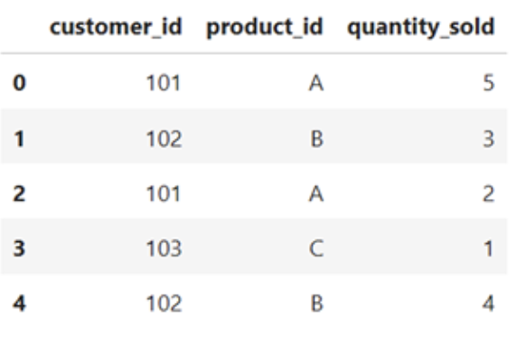
}

# Merging duplicates by aggregating values
merged_df = df.groupby(['cutomer_id', 'product_id']).agg({'quantity_sold': 'sum'}).reset_index()

merged_df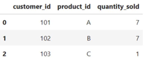

Addressing inconsistencies

Different types of inconsistencies will require different solutions. Inconsistencies resulting from incorrect data inputs or from typos may need to be corrected by a knowledgeable source. Alternatively, the incorrect data may be replaced using imputation, as if it were a missing value, or removed from the dataset entirely, depending on the circumstances.

Inconsistencies in the formatting of the data can be corrected using some standardizing methods. To remove leading and trailing spaces from a string, you can use the .strip() method. The .upper() and .lower() methods will standardize the case in strings. And converting dates to datetimes using pd.to_datetime will standardize date formatting.

You can also ensure every value in the column of a DataFrame is the same data type using the .astype() method.

Other formatting inconsistency corrections you may need to conduct include:

• Unit conversion
• Email, phone, and address standardization
• Removing punctuation from strings
• Using value mapping to address common abbreviations

value_mapping = {'M': 'Male', 'F': 'Female'}
standardized_value = value_mapping.get('M', 'Unknown')

Data Transformation and Feature Engineering

Data transformation and feature engineering are preprocessing techniques for transforming raw data into a format that is more suitable for machine learning algorithms and statistical analysis. In this section, we'll briefly explore some common data transformation and feature engineering techniques in Python.

Normalization and standardization

Normalization and standardization are two techniques used to bring features to a similar scale, which is important for many machine learning algorithms.

Normalization scales the data to a fixed range, usually between 0 and 1. This ensures that all features are on the same scale and prevents certain features from dominating others due to their larger magnitude.

from sklearn.preprocessing
 
import MinMaxScaler scaler = MinMaxScaler()
scaled_data = scaler.fit_transform(data)

Standardization, on the other hand, transforms the data to have a mean of 0 and a standard deviation of 1. This technique is useful when the data has different scales and varying ranges, and it ensures that each feature has a comparable impact on the model.

from sklearn.preprocessing
 
import StandardScaler scaler = StandardScaler()
standardized_data = scaler.fit_transform(data)

The specific characteristics of your data and the requirements of your intended model will dictate how you will scale your data.

Encoding categorical variables

Encoding categorical variables is an essential preprocessing step in machine learning when dealing with features that are not numerical. Categorical variables represent qualitative data, such as types, classes, or labels. To use these variables in machine learning algorithms, they need to be converted into a numerical format.

One common technique for encoding categorical variables is one-hot encoding, which transforms each category into a binary vector. This method is particularly useful when dealing with nominal categorical variables, where there is no inherent order or hierarchy among the categories.

import pandas as pd
encoded_data = pd.get_dummies(data, columns=['categorical_column'])

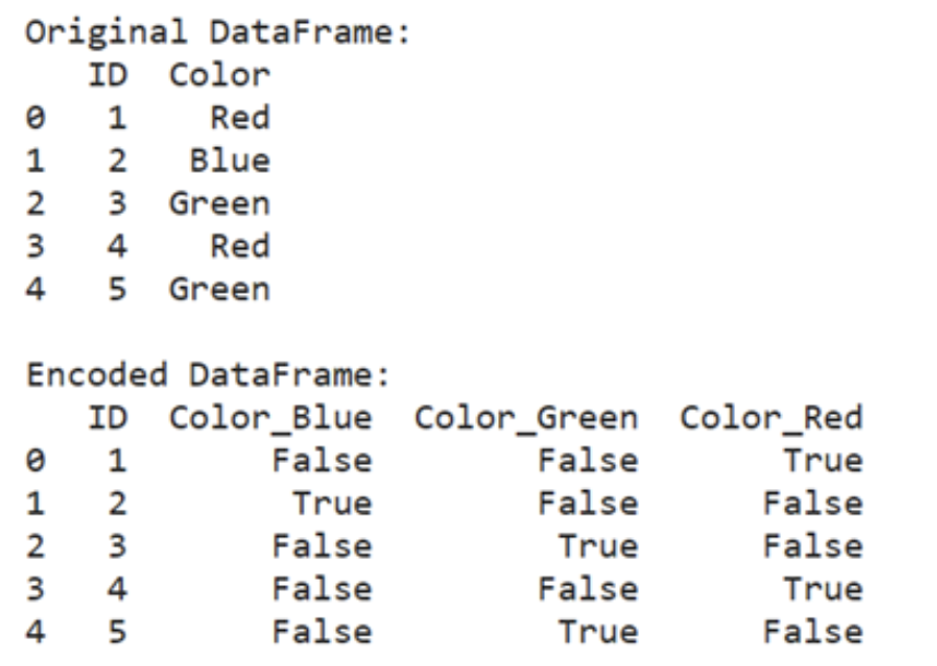
import pandas as pd

#Create a sample DataFrame with categorical column 
data = {
    'ID' : [1, 2, 3, 4, 5]
}
df = pd.DataFrame(data)

#Performe one-hot encoding 
encoded_data = pd.get_dummies(df, columns==['Color'])

print("Original DataFrame")
print(df)
print("\nEncoded DataFrame:")
print(encoded_data)

Another approach is label encoding, which assigns a unique integer to each category. Each category is mapped to a numerical value, effectively converting categorical labels into ordinal numbers. This method is suitable for ordinal categorical variables, where there is a natural order or ranking among the categories.

from sklearn.preprocessing import LabelEncoder
encoder = LabelEncoder()
encoded_data['categorical_column'] = encoder.fit_transform(data['categorical_column'])

from sklearn.preprocessing import LabelEncoder
import pandas as pd

#Create a sample DataFrame with categorical column 
data = {
    'ID' : [1, 2, 3, 4, 5]
    'Color' : [ 'Red', 'Blue', 'Green', 'Red', 'Green' ]
}
df = pd.DataFrame(data)

#Perform label encoding
encoder  = LabelEncoder()
df ['Color_LabelEncoded'] = encoder.fit_transform(df['Color'])

print("Original DataFrame:")
print(df[['ID', 'Color']])
print("\nDataFrame with Label Encoded Column:")
print(df[['ID', 'Color_LabelEncoded']])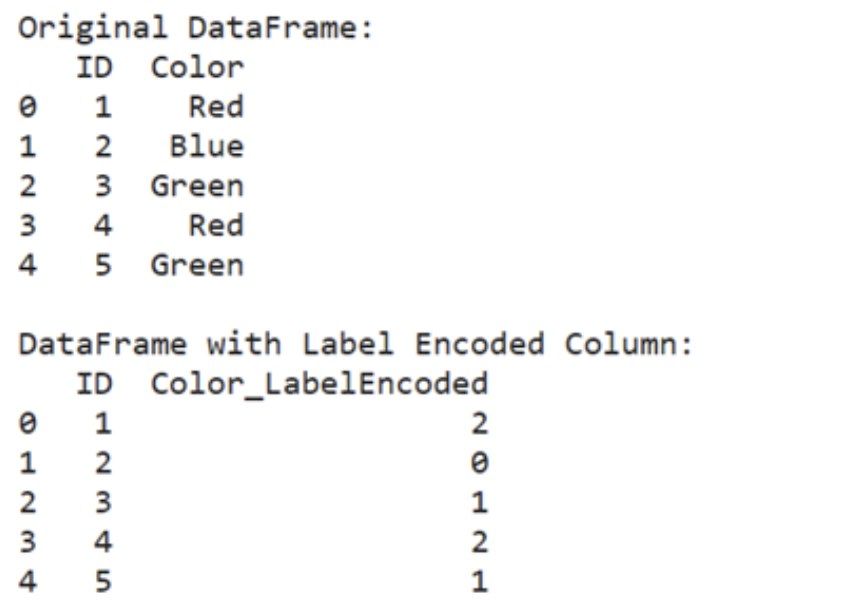

It's important to choose the appropriate encoding method based on the nature of the categorical variable and the requirements of the machine learning algorithm. One-hot encoding is generally preferred for nominal variables, while label encoding is suitable for ordinal variables.

Feature engineering techniques

Feature engineering is a step in machine learning model development involving the creation of new features or the modification of existing ones. This process is common when the raw data lacks features that directly contribute to the learning task or when the existing features are not in a form that the learning algorithm can effectively use.

Consider a scenario where you're working with a dataset of housing prices, and you want to predict the sale price of houses based on various features such as the number of rooms, square footage of the living area, and condition of the property. However, the dataset doesn't include a feature that directly captures the overall condition of the house.

In this case, you can create a new feature by combining existing features or extracting relevant information.

For example, you might create a feature called "Overall Condition" by aggregating the condition ratings of individual components of the house, such as the condition of the kitchen, the quality of the basement, the age of the property, recent renovations, etc.

In cases where the relationship between features and the target variable is nonlinear, polynomial features can be generated by raising existing features to various powers. This approach helps capture complex relationships between variables that may not be linearly separable.

from sklearn.preprocessing import PolynomialFeatures
poly = PolynomialFeatures(degree=2)
polynomial_features = poly.fit_transform(data)

In other cases, you may be dealing with high-dimensional datasets or multicollinearity among features. Techniques like Principal Component Analysis (PCA) can be employed to reduce the dimensionality of the dataset while retaining most of the relevant information.

from sklearn.decomposition import PCA
pca = PCA(n_components=2)
transformed_features = pca.fit_transform(data)

Feature engineering ensures that you have the correct data in the correct format for your model to use. There are many techniques in feature engineering, and which you use will be highly dependent on what you are trying to accomplish.

Check out this feature engineering course for more techniques that may be useful for you.

Cleaning Data in Python: Best Practices and Tips

Data cleaning is a critical step in any data analysis or machine learning project. Here are some best practices to keep in mind as you streamline your data cleaning process:

Store raw data separately

Always keep the original!

This is the number one most important tip when cleaning data. Keep a copy of the raw data files separate from the cleaned and processed versions. This ensures that you always have a reference point and can easily revert to the original data if needed.

Personally, I always make a copy of the raw data file before any changes are made and affix the suffix “-RAW” to the file name so I know which is the original.

Document your data-cleaning code

Add comments to your code to explain the purpose of each cleaning step and any assumptions made.

Look out for unintended consequences

You’ll want to make sure your data cleaning efforts aren’t significantly changing the distribution or introducing any unintended biases. Repeated data exploration after your cleaning efforts can help ensure you are on the right track.

Keep a data cleaning log

If you have a long cleaning process or one that is automated, you may want to maintain a separate document where you record the details of each cleaning step.

Details such as the date, the specific action taken, and any issues encountered may be helpful down the road.

Remember to store this document somewhere easily accessible, such as in the same project folder as the data or the code. In the case of an automated, regularly updated pipeline, consider having this log be an automatic part of the data cleaning process. This will allow you to check in and make sure everything is functioning smoothly.

Write reusable functions

Identify common data cleaning tasks and encapsulate them into reusable functions. This allows you to apply the same cleaning steps to multiple datasets. This is especially helpful if you have company-specific abbreviations you want to map.

Use DataCamp’s Data Cleaning Checklist to ensure you don’t miss anything!

Conclusion

Data cleaning is not just a mundane task; it's a crucial step that forms the foundation of every successful data analysis and machine learning project. By ensuring that your data is accurate, consistent, and reliable, you lay the groundwork for making informed decisions and deriving meaningful insights.

Dirty data can lead to erroneous conclusions and flawed analyses, which can have significant consequences, whether you're splitting candies among friends or making business decisions. Investing the time and effort into cleaning your data pays off in the long run, ensuring that your analyses are trustworthy and your results are actionable.

For more information and interactive exercises, check out DataCamp’s data cleaning course. For a hands-on challenge, try out this data cleaning code-along.