How to Lock Cells in Excel: Step-by-Step Guide to Protecting Your Data

Sometimes, we want to make sure certain parts of our spreadsheet don’t get changed by mistake. To do so, we can lock cells. It is a helpful way to protect things like sensitive data and the structure of our worksheet.

It’s different from tools like Freeze Panes (which just keep parts of your sheet visible while you scroll) or Data Validation (which helps control what data gets entered). In this article, I’ll walk you through how to lock all cells and also how to lock just the important ones, or even how to lock only the formula cells.

How to Lock All Cells in Excel

By default, all cells in Excel are locked, but that doesn’t mean they’re protected until you turn on sheet protection.

To confirm all the cells are locked, press Ctrl + A or the All button to select the whole sheet. Right-click and choose Format Cells (or press Ctrl + 1), go to the Protection tab, and make sure the Locked box is checked (which means all cells are locked). It usually is, but it's good to confirm.

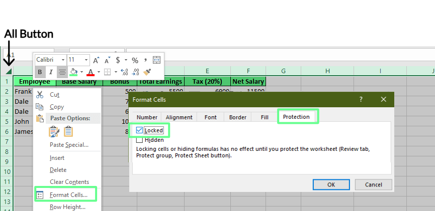
Checking locked cells. Image by Author.

Now, to lock the sheet from editing, go to the Review tab and click Protect Sheet. Enter the password (it will ask twice), and don’t forget this password because there’s no way to recover it later.

Below, you can see options for what we can still do, like selecting cells or formatting rows. Pick what you want to allow, then click OK. Now, the sheet is protected. All cells are locked, and users can only do what we allow.

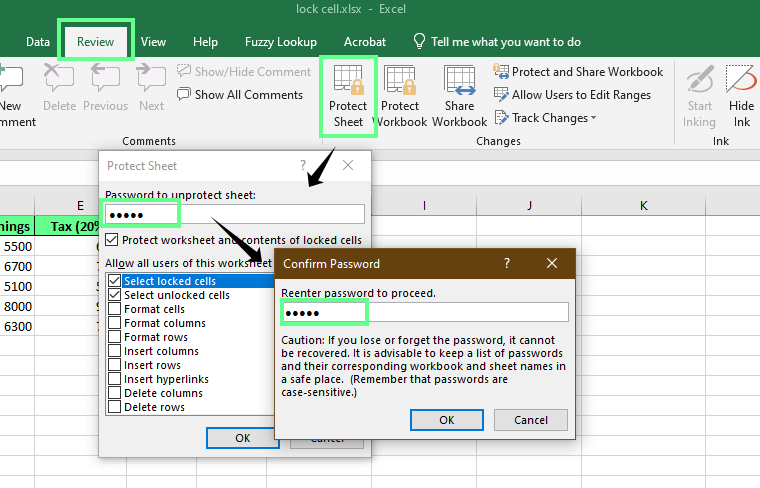
Protect the sheet with a password. Image by Author. 

How to Lock Specific Cells

Let’s say we’re working on a template or a shared spreadsheet and only want specific cells to be locked, like cells with formulas or key inputs, so users don't edit those cells. 

To do that, repeat the above Protection tab steps, but this time uncheck the Locked box and click OK. 

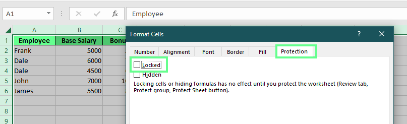
Locking specific cells. Image by Author

Next, select the cells you want to lock (in my case, it is E2:E6). Check the Locked box in the Protection tab and click OK and protect the sheet to lock it. You’ll see all the cells are unlocked except the ones we locked.

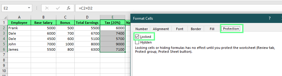
Specific cells locked. Image by Author

How to Lock Formula Cells

If we share a spreadsheet where people have to enter their data, it’s a good idea to lock the formula cells. That way, our background formulas stay safe, and no one can accidentally break them while typing in their info.

To lock formula cells, uncheck the Locked box to unlock all the cells under the Format Cells option (discussed above). Then, go to the Home tab and click the Find & Select option under the Editing group or press Ctrl + G. Next, click Special, choose Formulas, and click OK. 

Now the formula cells are selected. Select all the cells, press Ctrl + 1, and check the Locked box — now only formula cells are locked. You can also check the Hidden box if you want to hide those cells. 

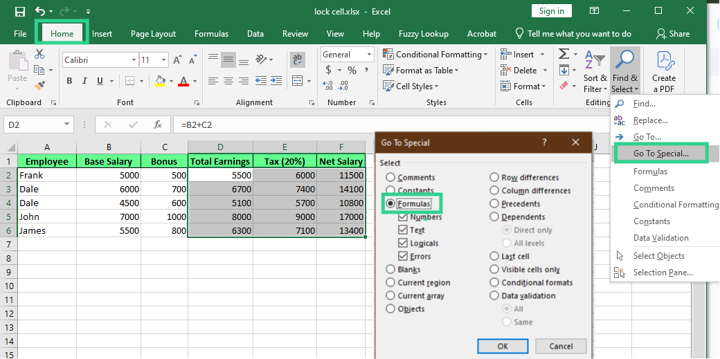
Lock the formula cells. Image by Author.

How to Unlock Ranges for Specific Users

Let’s say we have two people, and we want each to edit a different part of the same Excel sheet. For this, we can use a built-in feature, Allow Users to Edit Ranges.

Suppose the marketing team needs to fill in expenses, and the finance team needs to approve totals. We can unlock specific ranges for each of them and keep everything else protected.

1. Access the Excel ribbon

• Go to the Review tab.
• Click Allow Users to Edit Ranges.
• In the box that pops up, click New.

2. Set up the marketing section

• In the New Range window, name the range (like MarketingInput).

• In Refers to cells, type A2:C6.

• Choose a password, something like mkt123, and click OK.

• Confirm the password when prompted.

3. Add the finance section

• Repeat the same steps.

• Name this one FinanceApproval.

• Use D2:D16 for the cell range.

• Set a different password like fin456 and confirm it.

Now, like we did before, protect the sheet so the locked ranges work. Anyone can open and view the sheet. But if someone tries to edit the marketing section, they’ll need the marketing password. Same for finance — no password, no edits.

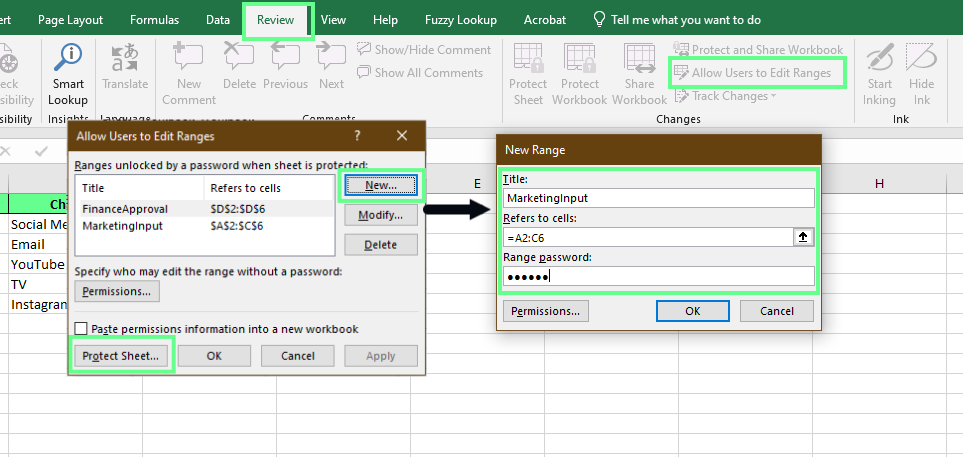
Lock specific ranges using the Allow Users to Edit Range option. Image by Author.

But typing in a password everytime you want to edit a range may be frustrating and time-consuming. If you’d rather give access to specific people without needing passwords, you can use the Permissions option instead. It’s quicker and smoother for teams who log in with usernames or email addresses.

Here’s how to set it up:

Access the Excel ribbon

• Go to the Review tab and click Allow Users to Edit Ranges.
• Click New, name your range, and pick the cells you want to unlock.

Add people instead of passwords

• Click Permissions.
• Hit Add, then type the usernames or email addresses of those who should have access. (I used Administrator as an example.)
• Click Check Names, then OK.
• If anything’s not working, click Advanced to fine-tune user settings.
• Tick the Edit range without a password box.

Once everything is set, click Protect Sheet, choose a password, and hit OK. Now, only allowed users can edit the range and won’t be interrupted with password prompts every time.

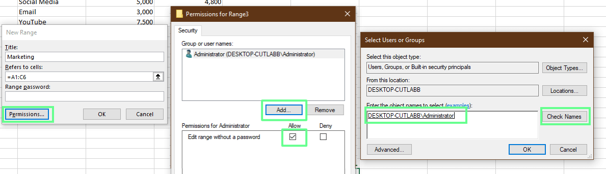
Permit specific rage without a password. Image by Author.

What Sheet Protection Settings Can Control

When we protect a sheet in Excel, we see a section called Allow all users of this worksheet to. This is where we decide what users can still do, even while the sheet is protected.

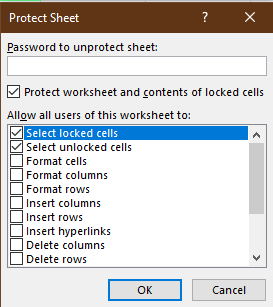
Protect sheet settings. Image by Author.

By default, everything is locked. So, if we want users to be still able to do specific tasks like formatting, deleting, or inserting, we’ll need to check those boxes.

Let’s see what each option means and why it matters:

Before you finish setting up protection in Excel, here are some quick reminders to help you avoid common mistakes:

• Spreadsheet protection stops others from accidentally changing things. But they can see all the confidential information. They can easily access your data if they know tools like VBA to bypass the protection. That’s why I recommend not keeping sensitive data in a shared spreadsheet. 

• Don't forget your password if you set one to protect your sheet. Excel doesn’t have a built-in way to recover passwords. This means once it's lost, you can’t change the protected areas anymore. So save it somewhere safe. 

• Always unlock the input fields before protecting the sheet. If users are supposed to type into specific cells, those cells need to be unlocked first. If you skip that step, users won’t be able to enter anything, and they may think something's broken.

When to Use Alternatives

Locking cells protects key parts of our sheet, like formulas. But other tools may be a better fit depending on what we’re trying to do.

Freeze Panes in Excel doesn’t protect your sheet. It keeps certain rows or columns visible while you scroll. This is perfect for long spreadsheets where we want to keep headers in sight as we move down the page.

Then there's the Data Validation tool. It doesn’t stop people from editing a cell, but guides what they can enter. We can set rules to only allow numbers, dates, or values from a dropdown list. It helps avoid typos and keeps data clean.

Final Thoughts

Locking cells in Excel is an easy way to stop others from changing important parts of our sheet. We can use it to protect formulas, control input areas, and manage who can edit what.

But don’t stop here. Test out the different options, and combine them with tools like Data Validation or Freeze Panes to keep your spreadsheet clear, accurate, and easy to use. Finally, don't forget to advance your career by taking our Excel Fundamentals skill track.