
Track
Data Analysis with Excel Power Tools
9 hr
Have you ever struggled to keep headers visible while scrolling through a large Excel sheet? I’ve been there, but that was before I knew about Freeze Panes. It’s a simple tool, but it makes a huge difference.
In this article, I will walk you through step-by-step instructions on using this feature to make your worksheet manageable. If you’re new to Excel, or if you have experience but still want to learn more, enroll in our comprehensive Excel Fundamentals skill track, which includes techniques to make you efficient and also includes a lot more, like data analysis methods, formula mastery, and effective visualization strategies.
If you are in a rush, let me give you the quick version. For the specific cases, keep reading below.
Freezing panes in Excel is a great way to keep specific rows or columns visible while you scroll through your worksheet. It’s helpful when you’re working with large datasets and want to keep things like headers or important labels in view. We can freeze multiple columns and rows, just the top rows and top columns, and also unfreeze them.
Now, if I want to freeze only the first row, which is usually the header of the dataset, I will go to the View tab under the Freeze Panes and click Freeze Top Row. Once we do this, we’ll see a grey line below the row, which indicates that the row is frozen and will stay in place as you scroll down.
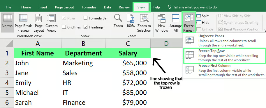
The top row is frozen. Image by Author.
If I want the first column to stay visible while scrolling horizontally, I will select the Freeze First Column option. A grey line will indicate that the first column is frozen.
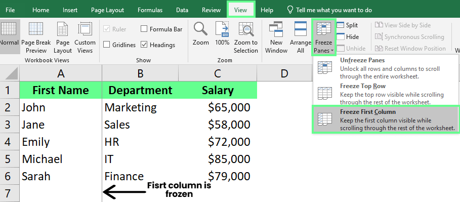
Freeze the first column. Image by Author.
To keep the first row and column visible while moving around the sheet, I’ll select any cell below those rows and to the right of those columns. Then, I’ll go to the View tab on the ribbon, click Freeze Panes, and choose Freeze Panes from the dropdown menu.
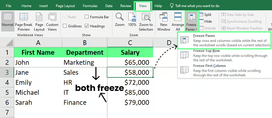
Freeze rows and columns. Image by Author.
Apart from locking the top row or the first column, sometimes, we have to freeze multiple rows, multiple columns, or even both rows and columns simultaneously. Let me explain how you can do so.
We have a sample dataset below. Now, if we want to freeze the first two rows, we’ll click on the first cell in Row 3. Then, we’ll go to the View tab on the ribbon. Click Freeze Panes, and then choose Freeze Panes from the dropdown list.
Now, the top two rows will stay visible as we scroll through the rest of the sheet.
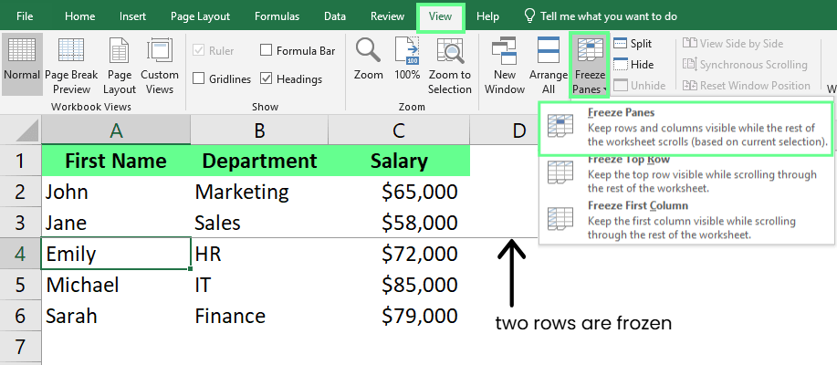
Freeze multiple rows. Image by Author.
To keep multiple columns visible while scrolling sideways, click on the column next to the last column you want to freeze. For example, if you want to freeze the first two columns (A and B), click on the first cell in Column C. Then, go to the View tab on the ribbon, click Freeze Panes, and select Freeze Panes from the dropdown menu.
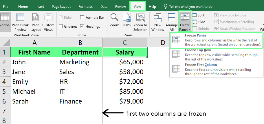
Freeze multiple columns. Image by Author.
Now, if you want to remove the frozen panes, go to the View tab > Freeze Panes, and click Unfreeze Pane.
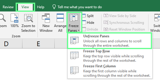
Unfreeze the panes. Image by Author.
This will remove all frozen rows and columns, and we can scroll freely again.
Some people confuse Split Panes with Freeze Panes. Here's a quick look at the difference between the two: Freeze Panes lets you lock specific rows or columns in place while you scroll. I use this feature whenever I want to keep my headers in view. It makes it much easier to track where I’m entering data, as I don’t have to scroll up and down to check the headers.
Split Panes are similar to Freeze Panes but work a little differently. They let you split the Excel screen into two or four sections, and you can scroll each section independently. We can use this to compare data from different parts of our spreadsheet without constantly scrolling back and forth.
I recently used Split Panes while working on a spreadsheet with over 500 rows. I wanted to compare data in Row 2 with the data in Row 400, and scrolling all the way down wasn’t practical. Split Panes made it so easy — I could see both rows side-by-side without any hassle.
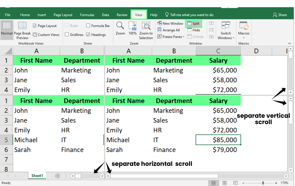
Split Pane. Image by Author.
Here, you can see how my sheet is split into four sections. This makes comparing data and keeping track of my work much easier, without getting lost or having to scroll too much. There's always more to learn with Excel. You would be surprised what you pick up with our Excel Fundamentals skill track or our Advanced Excel Functions course.
If you've already set up Freeze Panes in your Excel sheet, combining it with filtering and sorting can simplify data analysis. Let me show you how:
Let’s say I’m managing a Team Attendance Sheet with hundreds of rows, and I want to focus on only a few key pieces of data while keeping everything organized and easy to read. I can do this in a few different ways:
First, I’ll use the filter to narrow things down. To do this, I select any cell, go to the Data tab, and click Filter. This will add small arrows to the header row. Now, I can click the arrow in the Department column and choose Marketing. Then, in the Leaves Taken column, I’ll select Number Filters → Greater Than and type 5. This will filter the data, so I can only see the employees in Marketing who have taken more than five leaves.
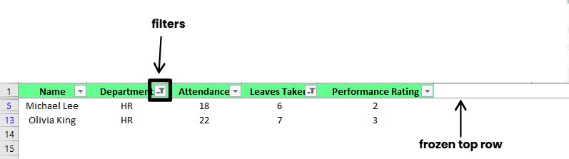
Freeze pane with filter. Image by Author.
With Freeze Panes already set up, my header row stays visible no matter how far I scroll down.
Now that the data is filtered, I can sort it for more valuable insights. Let’s say I want to see the employees with the highest Performance Rating at the top. To do so, I click the arrow in the Performance Rating column and choose Sort Largest to Smallest. This sorts the employees from the highest to the lowest rating, helping me quickly spot the top performers.
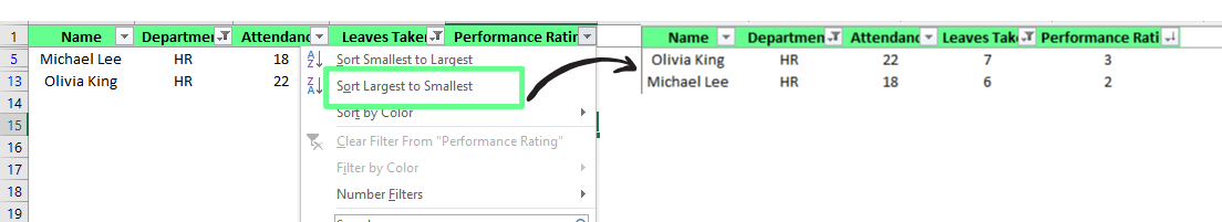
Freeze panes with sort. Image by Author.
By combining Freeze Panes with filtering and sorting, I can keep my data organized and focus on the most important information without losing track of the bigger picture.
Recently, I was working on a spreadsheet with a big PivotTable, and it was so hard to see the column headings when I scrolled down. So, I froze the top rows, just like you would in any other Excel sheet. I clicked on a cell in the row directly below the top row of the PivotTable, then went to the View tab, clicked the Freeze Panes dropdown, and selected Freeze Panes. This way, the top rows remained visible as I scrolled through the data.
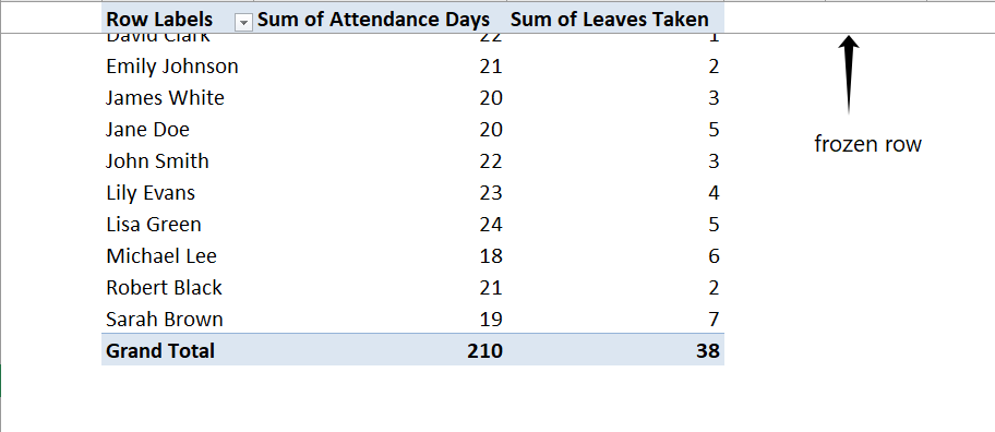
Freeze top rows in PivotTable. Image by Author.
Let’s look at common issues and their solutions to help you avoid similar problems with Freeze Panes.
I first selected the wrong cell while freezing panes. I didn’t realize the cell you choose determines what stays visible. So, the key is to select the cell directly below the rows and to the right of the columns. Excel freezes everything above the chosen cell and to its left.
I once wanted to freeze Row 33, so I selected Row 34 and used the Freeze Panes option. But instead of freezing Row 33, Excel froze Row 10, and I couldn’t figure out why. But now I know: That happened because Excel only freezes rows starting from the top of the sheet, and it depends on what’s visible on your screen. If rows above the one you’re trying to freeze aren’t visible, Excel won’t include them. Here’s how I fixed it: I made sure Rows 1–33 were visible on my screen, then selected Row 34 and used Freeze Panes again. This time, it worked perfectly, and Rows 1–33 stayed frozen as I scrolled down.
Once, I was surprised to see that the Freeze Panes option in Excel was greyed out. After some digging, I realized Freeze Panes only works in Normal View. So, I checked under the View tab and noticed I was in Page Layout. I immediately switched back to Normal View, and the option became available.
Freeze Panes makes working in Excel much easier. It saves time, keeps everything organized, and helps us compare data without hassle. If you want to sharpen your skills in Excel, check out our courses, such as Data Analysis in Excel, Data Preparation in Excel, and Data Visualization in Excel.
Once you're comfortable with Excel, you can take the next step and prepare for your interview by practicing with our top 30 Excel interview questions.
Gain the skills to maximize Excel—no experience required.
Learn Excel with DataCamp
Track
Course
Course
Tutorial
Allan Ouko
Tutorial
Laiba Siddiqui
Tutorial
Laiba Siddiqui
Tutorial
Laiba Siddiqui
Tutorial
Javier Canales Luna
Tutorial
Allan Ouko