Index Match Excel: A Better Way to Look Up Data

INDEX MATCH, a combination of the two Excel functions, INDEX() and MATCH(), is an alternative to the commonly used VLOOKUP() function.

In this guide, I will walk you through how INDEX() and MATCH() work individually and together, how to perform vertical and horizontal lookups, and best practices for using INDEX MATCH with practical examples.

What Is INDEX MATCH in Excel?

INDEX MATCH is a shorthand way to refer to the nesting of the two functions. It is equivalent to the idea of INDEX(MATCH()). Let’s see how both work individually and together.

INDEX() function in Excel

The INDEX() function in Excel returns a value or a reference to a value from within a range or table. You can use it in two ways: array form and reference form.

Array form

You can use the array form when you're working with a fixed table or array. In this format, INDEX() pulls out a value based on the row and column number you specify. Its syntax is:

INDEX(array, row_num, [column_num])

Let’s understand these arguments:

• array (required) is the range or array of values you’re working with.

• row_num (required) is the row number from which to return a value.

• column_num (optional) is the column number from which to return a value.

We must specify at least one, either row_num or column_num so Excel can locate the value.

However, here are some quick notes you should keep in mind when working with this syntax:

• If the array has only one row or column, you can skip row_num or column_num.

• If both row_num and column_num are included, INDEX returns the value where they intersect.

• If you set row_num or column_num to 0, Excel returns the entire column or row (you’ll need to enter it as an array formula to see the result).

Reference form

You can use the reference form when working with multiple ranges and need to specify which one to look at.

Its syntax is:

INDEX(reference, row_num, [column_num], [area_num])

Let's understand these arguments:

• reference (required) is used to reference one or more cell ranges.

• row_num (required) is the row number in the selected area.

• column_num (optional) is the column number in the selected area.

• area_num (optional) tells Excel which range to use if there’s more than one.

Here are some additional points that you must remember:

• If area_num is left out, Excel uses the first range by default.

• You can’t mix ranges from different sheets in this form; it will trigger an error.

• If both row and column are omitted, it returns the full specified area.

MATCH() function in Excel

The MATCH() function helps you find the position of a value in a row or column. Instead of returning the value itself, it tells you where it is in the list.

Its syntax is:

MATCH(lookup_value, lookup_array, [match_type])

Let’s understand these arguments:

• lookup_value (required) is the value you want to find. It can be a number, text, logical value (TRUE/FALSE), or a reference to a cell.

• lookup_array (required) is the range of cells Excel will search through.

• match_type (optional) defines how Excel looks for the match. The default is 1. Here 1 finds the largest value less than or equal to lookup_value (requires ascending order). 0 finds the exact match (any order). -1 finds the smallest value greater than or equal to lookup_value (requires descending order).

The MATCH function is not case-sensitive, so it treats uppercase and lowercase letters the same. If you’re working with text and want to use wildcard characters like * (any number of characters) or ? (a single character), make sure to set match_type to 0. Because that’s the only mode that supports wildcard search.

How Do INDEX() and MATCH() Work Together in Excel?

One of the most common uses of MATCH() is pairing it with the INDEX() function. While MATCH() finds the position of a value, INDEX() retrieves the value at that position. 

Nesting MATCH() inside INDEX() gives you a formula that’s dynamic and resilient when columns or rows shift over time. 

For example, I have a sample dataset. And if I want to find out what is in the same row in column B as that of Banana in column A, I can use INDEX MATCH together like this:

=INDEX(B2:B5, MATCH("Banana", A2:A5, 0))

Here, MATCH("Banana", A2:A5, 0) finds the position of Banana in column A and INDEX(B2:B5, ...) returns the value from the same row in column B.

INDEX MATCH vs. VLOOKUP(): Which One Should You Use?

INDEX MATCH can do jobs that VLOOKUP() can’t. However, choosing between them depends on the level of flexibility and performance you require in your Excel sheets. Let’s compare them.

Column flexibility and data integrity

One of the biggest drawbacks of VLOOKUP() is its reliance on fixed column numbers. If you insert or move columns, your formula can break.

Take this example:

If a new column is added between Column A and Column B, the third column shifts, and the formula returns incorrect results, as you can see in the image below.

=VLOOKUP("Apple", A2:C5, 2, FALSE)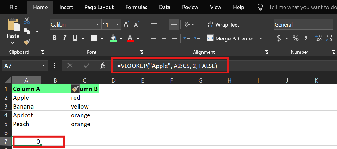

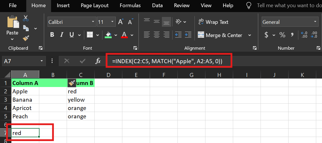
INDEX MATCH avoids this issue by working with defined ranges instead of hardcoded column positions:

=INDEX(B2:B5, MATCH("Apple", A2:A5, 0))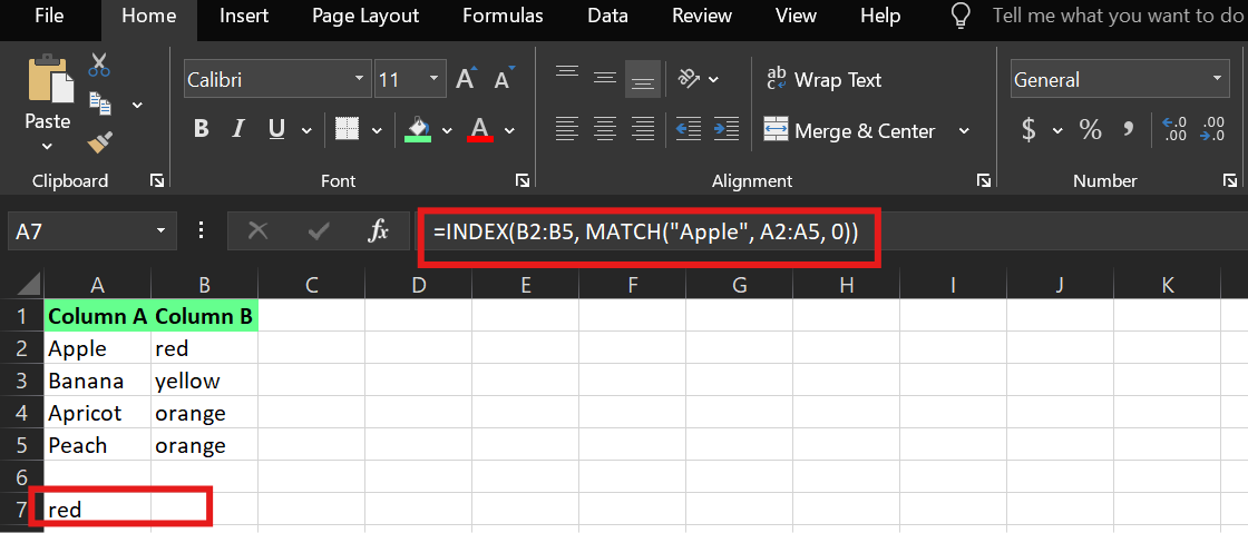

Even if columns are rearranged, this formula remains effective, which makes it more reliable and easier to maintain. Here, a column is inserted before column B; the formula is updated automatically, and the results remain correct. This is the magic of an INDEX MATCH.

Lookup direction and versatility

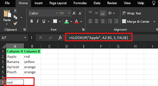
VLOOKUP() can only search left to right. That means your lookup column must always be the first in your range. If the value you need is on the left of the lookup column, VLOOKUP() can’t find it.

However, if we look up by the fruit name to find its color on the right, this formula will work. For example, if we want to find the color of a banana from our list, it gives the accurate result: 

With INDEX MATCH, that limitation doesn’t exist. You can search in any direction: left, right, up, or down. It also supports horizontal lookups to give you more control over how you organize your data. 

Let’s apply INDEX MATCH to this example and see how it allows both left and right lookups.

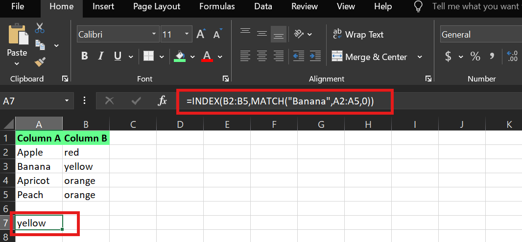
For left lookup, you can use the following formula, and it will give the accurate output: 

=INDEX(A2:A5, MATCH(“yellow”, B2:B5,0))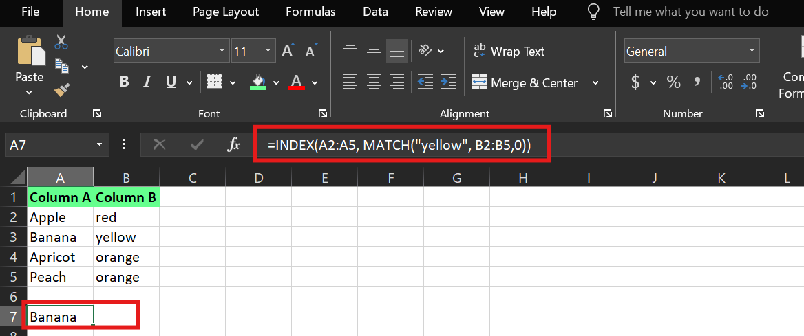

For the right lookup, you can use the following formula, and it will give the correct output: 

=INDEX(B2:B5, MATCH(“Banana”,A2:A5,0))

Performance and efficiency in Excel

VLOOKUP() scans the entire table to find a match and retrieve a value in one go. But INDEX MATCH splits the task: MATCH() finds the row or column, and INDEX() retrieves the value. 

This makes it faster and more memory-efficient, especially in complex or high-volume workbooks.

Here is a table to give you a better idea of which function supports what functionality:

When to use INDEX MATCH

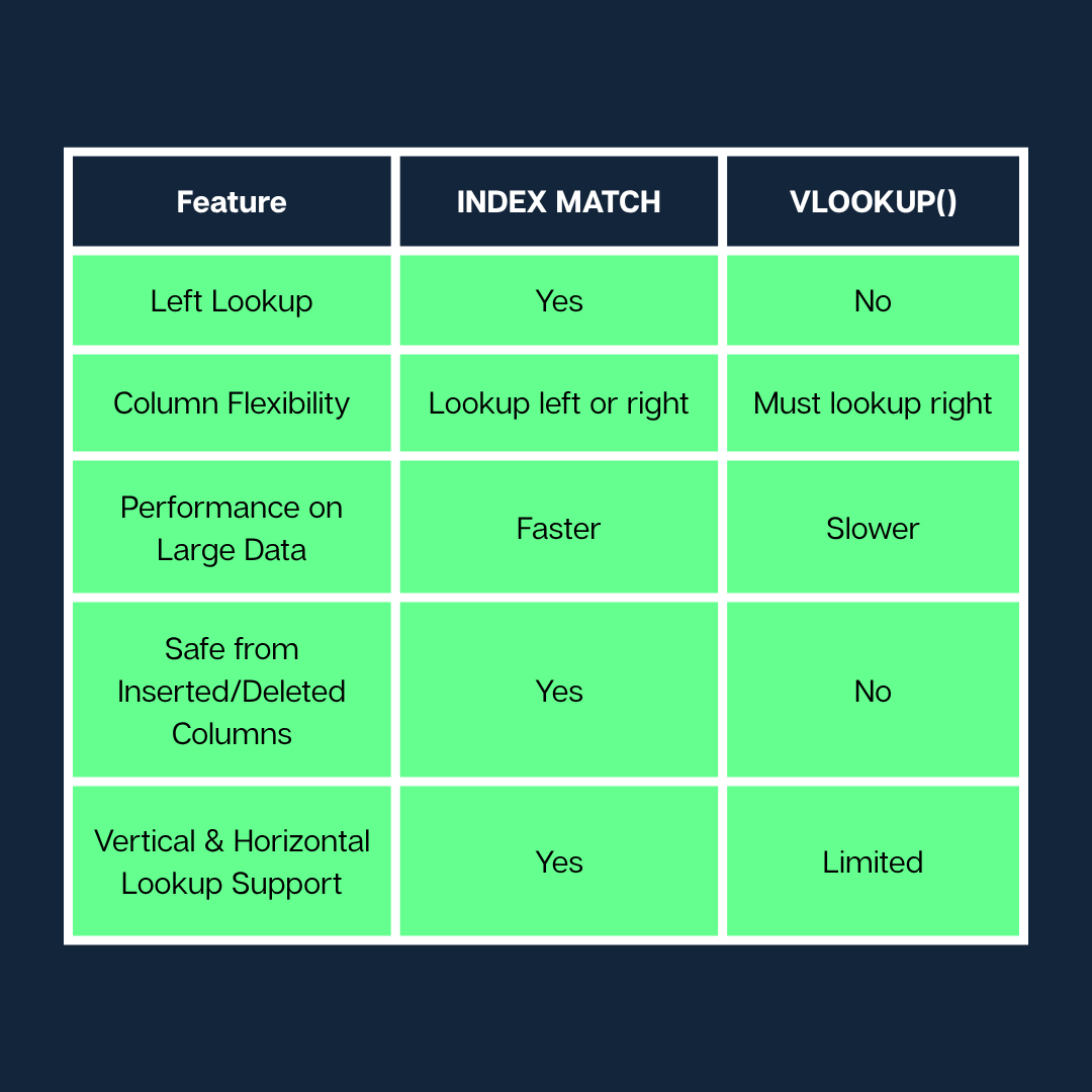
You can use INDEX MATCH when:

• You’re working with large datasets where speed matters
• Your model is dynamic, with columns being added or rearranged
• You need to look up values to the left or in horizontal ranges

If your Excel files are small and simple, VLOOKUP() may still do the job. But for advanced modeling and reporting, INDEX MATCH is a safer bet.

How to Use INDEX MATCH Step-by-Step

Let’s say you’ve two columns: Fruits and Sales. You want to find the sales value for “Apple.”

For this, type the combined INDEX MATCH formula and press Enter:

=INDEX(B2:B6, MATCH("Apple", A2:A6, 0))

Here, MATCH("Apple", A2:A6, 0) finds the position of “Apple” in the Fruits list. And INDEX(B2:B6, ...) uses that position to return the corresponding sales value from the Sales column.

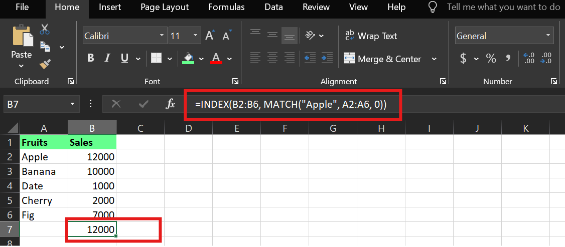
You can see the formula returned 12000, which is the sales value for Apple. So, that’s your result.

Avoiding INDEX MATCH Errors

While INDEX MATCH is a good combo, it can still throw errors if not set up correctly. Here’s how to troubleshoot the most common issues and avoid mistakes that could break your formulas.

#N/A errors and how to resolve them

The #N/A error means Excel couldn’t find the value you’re looking for. Some common causes behind this could be:

• Typos, extra spaces, or mismatched text (e.g., "apple" vs. "Apple")

• No value in the lookup range

• Wrong match_type, for example, 1 instead of 0 for an exact match

• Hidden characters (like non-breaking spaces) in the data

So there are two ways to fix this:

Use TRIM() to clean up leading or trailing spaces:

=MATCH(TRIM("Apple"), A2:A6, 0)

Add IFERROR() to show a fallback value instead of an error:

=IFERROR(INDEX(B2:B6, MATCH("Apple", A2:A6, 0)), "Not found")

#REF! errors in INDEX MATCH formulas

The #REF! error usually points to a broken reference—often because of:

• A mismatch between the number of rows in your INDEX() and MATCH() ranges

• Deleted rows or columns used in your formula

• Copying and pasting formulas without updating cell references

But there are some easy ways you can fix this: 

• Ensure the INDEX() and MATCH() ranges are the same size:

=INDEX(B2:B6, MATCH("Apple", A2:A6, 0))

• Lock ranges with absolute references (like $A$2:$A$6) to keep formulas stable during copy-paste.

• Avoid deleting cells that formulas depend on.

Slow performance and large data sets

If you’re working with thousands of rows, unoptimized INDEX MATCH formulas can slow Excel down.

Here’s how you can optimize it:

• Limit lookup ranges instead of referencing whole columns:

=INDEX(B2:B1000, MATCH("Apple", A2:A1000, 0))

• Avoid volatile functions like OFFSET(), INDIRECT(), and NOW() near your lookups.

• Use Excel Tables or named ranges to keep things organized and improve performance.

Managing spill errors in Excel 365

Excel 365 introduces dynamic arrays, which can “spill” results into adjacent cells. If there’s an issue with that process, you’ll get a #SPILL! error.

Some common causes could be:

• Adjacent cells are not empty.
• The formula returns multiple values into a blocked or merged cell range.
• You're using a dynamic array where only a single value is needed.

But these issues are fixable. Here’s how you can overcome them:

• Clear the cells below or beside the formula.
• Unmerge any cells in the spill area.
• If you only want one value, force a single result with @:

=@INDEX(B2:B6, MATCH("Apple", A2:A6, 0))

Final Thoughts

If you’ve been relying on VLOOKUP(), now’s the time to move to something more stable. You can start with a few simple lookups using INDEX MATCH in a copy of your working file. Try swapping in the new formula where column changes cause errors or where your data structure demands flexibility. Once you see how cleanly it handles those cases, it’ll be hard to go back.