How to INDEX MATCH Multiple Criteria in Excel

A couple of years ago, I worked on a marketing campaign analysis where I had to compare sales performance across multiple regions. The data was spread across multiple Excel sheets, and I had to pull specific product sales numbers into a single summary report. At first, I tried manually searching and copying the data, but it was not as easy as I thought. If there’s one wrong row, the whole report could fall apart.

That’s when I found INDEX MATCH(). It took me a few tries to get the formula right, but it became a part of my routine once I saw how easily it could locate and pull the exact numbers I needed. With only two functions, I could pull exactly the data I needed, no matter how scattered it was across spreadsheets.

In this article, I’ll explain how you can do the same using the INDEX() and MATCH() functions. There's always more to learn with Excel. If you are a beginner, I highly recommend our Introduction to Excel course. If you have more experience, try our Advanced Excel Functions course.

A Refresher on INDEX MATCH

INDEX MATCH is a shorthand way of talking about the combination of two Excel functions that work together to perform advanced lookups. We could also refer to this idea as INDEX(MATCH()), but I'll choose INDEX MATCH in this article. Now, let's take a look at each in turn:

The INDEX() function retrieves the value of a cell based on its position within a specified range. Here’s its syntax:

=INDEX(array, row_num, [column_num])

Here:

• array is the range of cells from which you want to retrieve a value.

• row_num is the row number in the array from which to return a value.

• column_num (optional) is the column number in the array from which to return a value.

The MATCH() function identifies the relative position of a value within a range. Its syntax is:

=MATCH(lookup_value, lookup_array, [match_type])

Here:

• lookup_value is the value you want to find.

• lookup_array is the range where the function searches for the value.

match_type is optional. 1 (default) finds the value less than or equal to lookup_value (array must be sorted in ascending order). 0 finds an exact match (array need not be sorted). -1 finds the smallest value greater than or equal to lookup_value (array must be sorted in descending order).

How to combine INDEX() with MATCH()

By nesting MATCH() within INDEX(), we can create a dynamic lookup. Let’s understand this with an example: Suppose you want to find the position of David Wilson in the dataset. Instead of hardcoding the row number in INDEX(), use MATCH() to determine it:

=INDEX(C2:C6, MATCH("David Wilson", A2:A6, 0))

In the above formula, MATCH("David Wilson", A2:A6, 0) returns 4, which is the row position. And INDEX(C2:C6, 4) retrieves the value from the 4th row of the range C2:C6, which is Seattle.

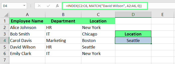
Combine INDEX() with MATCH(). Image by Author.

To make this even more dynamic, you can replace the hard-coded David Wilson with a cell reference. This way, the formula adjusts automatically based on the value in D4:

=INDEX(C2:C6,MATCH(D4,A2:A6,0))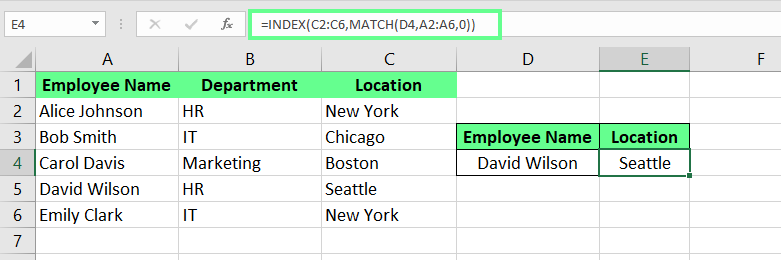

Replace the hardcoded value in the INDEX MATCH. Image by Author.

INDEX MATCH vs. VLOOKUP()

Now that you know how INDEX() and MATCH() work individually and how combining them makes lookups more dynamic, let’s see why INDEX MATCH is a better choice than VLOOKUP().

• Unlike VLOOKUP(), which requires the lookup column to be on the left, INDEX MATCH allows you to retrieve data from any column, regardless of its position.

• INDEX MATCH processes only the required range of cells compared to VLOOKUP(), which scans entire tables. 

• Formulas using VLOOKUP() can break if columns are inserted or deleted, as they rely on static column indices. On the other hand, INDEX MATCH references dynamic ranges to ensure your formulas remain intact despite structural changes to your data.

• With INDEX MATCH, we don’t have to count column numbers manually. Specify the lookup column and the return column, and you’re done. 

INDEX MATCH with Multiple Criteria

I often have to work on datasets that contain duplicate entries, and finding values in them is extremely difficult. But now I use INDEX MATCH because it handles these scenarios very easily, unlike other standard lookup formulas. Let me walk you through how I use this step by step.

Set up data for multiple criteria

First, create your dataset and make sure it is well organized into a table with clear headers for each column. Each row should represent a unique record, and each column should contain a specific data attribute.

For example, here’s a sample dataset:

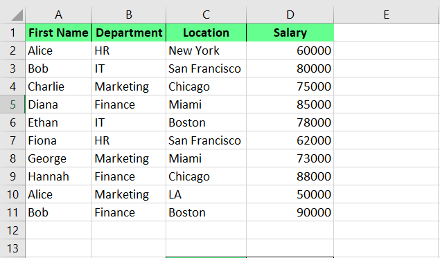
Dataset for INDEX MATCH multiple criteria. Image by Author.

Write the formula for multiple criteria

Once your data is properly organized, it’s time to write the formula. The INDEX MATCH formula retrieves a value from another column by identifying a row that meets multiple conditions. This is done by combining logical tests within the MATCH() function and embedding it inside the INDEX() function.

Here’s the basic syntax for this: 

{=INDEX(return_range, MATCH(1, (criteria1=range1) * (criteria2=range2) * (…), 0))}

Here: 

• Return_range is the range from which the value will be returned.

• Criteria1, Criteria2, … are the conditions to be satisfied.

• Range1, Range2, … are ranges corresponding to the criteria.

Now that we have a data set up, let's look closely at the two methods to answer our question: how to use INDEX MATCH with multiple criteria.

Use helper columns for complex criteria

If your dataset has multiple conditions, use helper columns to simplify the process. It will combine all conditions into a single column for easier lookups. For example, I am using the same dataset to create a helper column by combining the First Name and Salary columns:

=A2&B2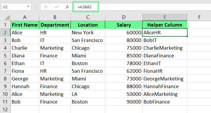

Create a helper column. Image by Author.

This helper column simplifies my INDEX MATCH formula. Instead of writing a complex array formula with multiple conditions, I referenced the helper column in my formula for a simpler approach:

=INDEX(D2:D11, MATCH("AliceHR", E2:E11, 0))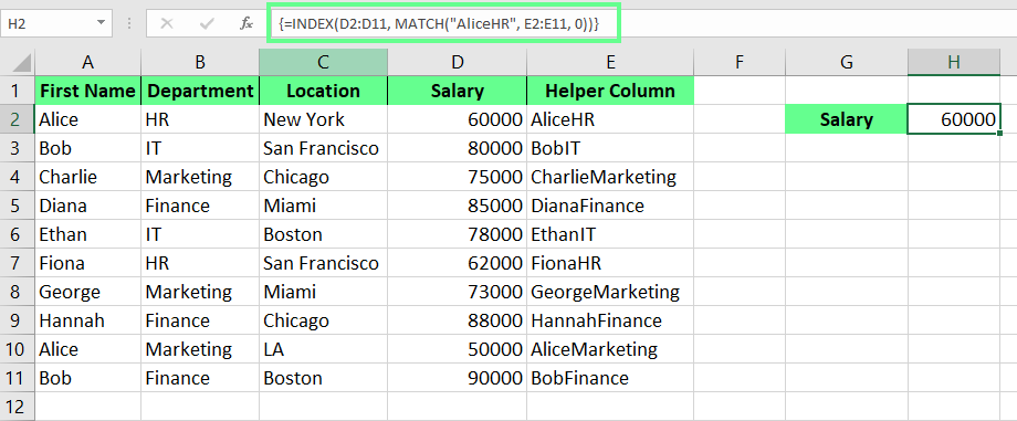

INDEX MATCH with helper column. Image by Author.

Combine multiple criteria with an array formula

If you don’t prefer helper columns, you can use array formulas to achieve the same result. They allow you to evaluate multiple criteria directly within the MATCH() function. For example, here’s how I find Alice’s Salary in the HR department:

Step 1: Write the MATCH() function with logical conditions:

 MATCH(1, (F4=A2:A11) * (F5=B2:B11), 0)

In this formula, 1 ensures the MATCH() function looks for rows where all conditions are true. (F4=A2:A11) checks if the value in F4 matches any value in the range A2:A11. (F5=B2:B11) checks if the value in F5 matches any value in the range B2:B11. The * operator acts as an AND logic, ensuring all conditions are met.

Step 2: Wrap this MATCH() function inside the INDEX() function:

=INDEX(D2:D11, MATCH(1, (F4=A2:A11) * (F5=B2:B11), 0))

Step 3: Finalize the formula. If you are using an older version of Excel, press Ctrl+Shift+Enter to make it an array formula. In newer versions, press Enter.

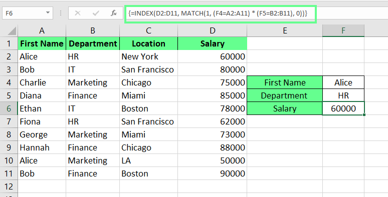
Array INDEX MATCH with multiple criteria. Image by Author.

Advanced Uses for INDEX MATCH with Multiple Criteria

You can do so much more with the INDEX MATCH function. Let’s see how: 

Use INDEX MATCH with named ranges and dynamic ranges

I use named ranges in Excel to set meaningful names like results or totalSales instead of standard references like A1:A10. This way, it becomes easier to manage formulas across different sheets. 

To name a cell range, select the cells and press Ctrl + F3 (for Windows) or Cmd + F3 (for Mac) to open the Name Manager. Then, Click New, enter a name, and click OK.

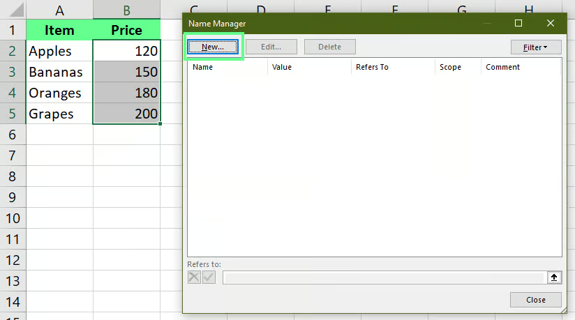
Name the range. Image by Author.

The only difference between a named range and a dynamic range is that a named range refers to a fixed group of cells, whereas a dynamic range automatically adjusts when data is added or removed.

To set a dynamic range, select the cells. On the Formulas tab, click Name Manager or press Ctrl + F3 to open the Excel Name Manager and click New. The New Name dialog box will appear. Now, in the Name field, enter your desired name. Then, in the Refers to field, input the formula for the dynamic range. 

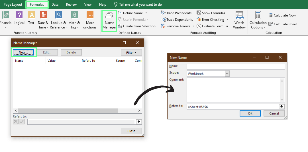
Set a dynamic range. Image by Author. 

Now let’s look at an example: I defined two dynamic and one static range:

• total_amount: =$F$2:INDEX($F:$F, COUNTA($F:$F))

• items_list: =$A$2:INDEX($A:$A, COUNTA($A:$A))

• lookup_value: =$I$3

Now, I use these ranges within the INDEX MATCH formula:

=INDEX(total_amount,MATCH(lookup_value,items_list,0))

And you can see the formula becomes much easier to understand with clear names.

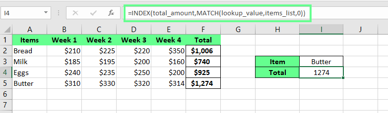
Use dynamic and named ranges with INDEX MATCH. Image by Author.

Nested INDEX MATCH for complex lookups

Apart from basic work, you can use nested INDEX MATCH functions to handle complex lookups too. For example, I have a dataset showing sales by product category across different regions. 

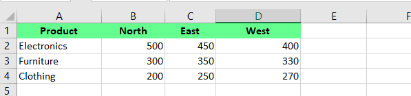
Raw dataset. Image by Author.

I want to find furniture sales in the East. But to do so, I’ve to match both the product category (row) and the region (column), which a basic INDEX MATCH can’t do. That’s why I use the following nested INDEX MATCH formula here:

=INDEX(B2:D4, MATCH(D6, A2:A4, 0), MATCH(D7, B1:D1, 0))

Here’s how it works: The INDEX() pulls a value from the range B2:D4, but it needs a row number and a column number to tell it exactly where to look. So, the first MATCH(D6, A2:A4, 0) figures out the row number. If D6 contains Furniture, it searches column A2:A4 and finds it in the second row.

Next, MATCH(D7, B1:D1, 0) determines the column number. If D7 says East, it looks across B1:D1 and finds it in the second column.

Once INDEX() knows the row and column, it displays the output values. In our case, the sales for Furniture in the East are 450.

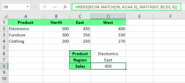
Use nested INDEX MATCH. Image by Author.

I use this formula instead of manually searching through rows and columns because it handles everything precisely. 

Common Challenges and Troubleshooting Tips

When I started using INDEX MATCH, I ran into several challenges, and I don’t want you to experience the same frustrations. So, I’ll walk you through the most common challenges and show you how to overcome them.

Handle errors in INDEX MATCH formulas

Errors like #N/A and #VALUE! can look frustrating initially, but they’re pretty easy to fix. Let’s see how to spot what’s causing the problem and the simple steps to solve it.

The #N/A error occurs when the MATCH() function doesn’t find a value. This is because the lookup value doesn’t exist in the search array, or the data contains hidden spaces. For example, I once referenced the wrong column while pulling Employee Names:

=INDEX(B2:B6,MATCH(E3,C2:C6,0))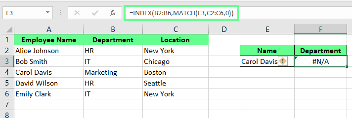

#N/A error in INDEX MATCH. Image by Author.

To fix such issues, confirm the lookup value exists in the array and use the TRIM() function to clean up spaces:

=TRIM(INDEX(B2:B6,MATCH(E3,A2:A6,0)))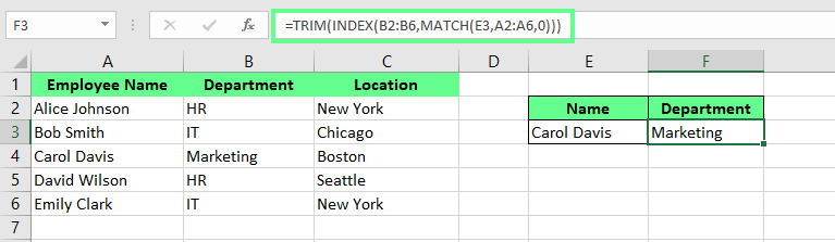

#N/A error fixed in INDEX MATCH. Image by Author.

#VALUE! error appears when the formula isn’t set as an array formula. For example, if I use the MATCH() function and include more than one range, Excel sees it as an array formula. However, if it’s not set up properly, Excel will throw a #VALUE! error.

=INDEX(C2:C6,MATCH(D4&E4,A2:A6&B2:B6,0))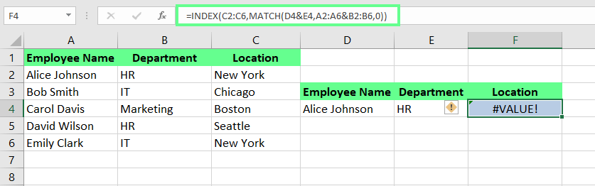

#Value error in INDEX MATCH. Image by Author.

To resolve it, press Ctrl + Shift + Enter after you’ve entered the formula. This way, Excel will wrap the formula in curly braces {}, indicating it’s now an array formula. But don’t type the braces manually because it will break the formula.

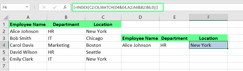
#Value error fixed in INDEX MATCH. Image by Author.

Optimize performance with large datasets

In larger datasets, my formulas slowed down from time to time, and because of this, I had to wait for calculations to update. If you’re also struggling with similar issues, try these tips: 

• Limit the lookup range: Restrict ranges to only what’s necessary. For example, instead of A:A, use A1:A100 to reduce computation time.

• Use helper columns: Pre-calculate complex criteria with helper columns. This will reduce the computational load of array formulas.

• Enable manual calculation mode: Switch Excel to manual calculation mode to avoid constant recalculations. After making changes, press F9 to update formulas manually.

• Avoid volatile functions: Minimize using volatile functions like NOW(), RAND(), and TODAY() in combination with INDEX MATCH. These functions trigger recalculations every time the workbook updates.

Final Thoughts 

INDEX MATCH techniques save time and simplify complex data analysis. If you work with massive datasets, they can be worth a try. But, the best way to solidify your understanding is through practice. So, I’d say tackle a few datasets and experiment with what you’ve learned. That’s how I sharpened my skills. 

To deepen your knowledge, check out our Advanced Excel Functions course to master a broader range of powerful tools. But if you want to build comprehensive expertise around data analysis in Excel, I’d recommend our Data Analysis in Excel course. It covers everything from data preparation to visualization.