Course
Introduction to Python
4 hr
6.9M
With the Exploratory Data Analysis (EDA) and the baseline model at hand, you can start working on your first, real Machine Learning model.
Note that this tutorial is based on a Facebook Live code along session; You can rewatch it here:
Before you get started, import all necessary libraries:
# Import modules
import pandas as pd
import matplotlib.pyplot as plt
import seaborn as sns
import re
import numpy as np
from sklearn import tree
from sklearn.model_selection import train_test_split
from sklearn.linear_model import LogisticRegression
from sklearn.model_selection import GridSearchCV

# Figures inline and set visualization style
%matplotlib inline
sns.set()

# Import data
df_train = pd.read_csv('data/train.csv')
df_test = pd.read_csv('data/test.csv')
data that consists of training and test sets combined. You do this because you want to preprocess the data a little bit and make sure that any operations that you perform on the training set are also being done on the test data set.# Store target variable of training data in a safe place
survived_train = df_train.Survived
# Concatenate training and test sets
data = pd.concat([df_train.drop(['Survived'], axis=1), df_test])
data using the info() method.data.info()
<class 'pandas.core.frame.DataFrame'>
Int64Index: 1309 entries, 0 to 417
Data columns (total 11 columns):
PassengerId    1309 non-null int64
Pclass         1309 non-null int64
Name           1309 non-null object
Sex            1309 non-null object
Age            1046 non-null float64
SibSp          1309 non-null int64
Parch          1309 non-null int64
Ticket         1309 non-null object
Fare           1308 non-null float64
Cabin          295 non-null object
Embarked       1307 non-null object
dtypes: float64(2), int64(4), object(5)
memory usage: 122.7+ KB
There are 2 numerical variables that have missing values.
What are they?
That's right, you're missing values for the 'Age' and 'Fare' columns! You see in the result of the .info() method above that you're missing 263 values for the first column, since you have only 1046 non-null values for the total of 1309 entries of your DataFrame. Ideally, you of course want all of those 1309 to have non-null values, but that isn't the case here!
Luckily, you're only missing one for the Fare column. Also notice that 'Cabin' and 'Embarked' are also missing values and you'll need to deal with that also at some point.
However, now you'll focus on fixing the numerical variables: you will impute or fill in the missing values for the 'Age' and 'Fare' columns, using the median of the of these variables where you know them.
Note that in this case, you use the median because it's perfect for dealing with outliers. In other words, the median is useful to use when the distribution of data is skewed. Other ways to impute the missing values would be to use the mean, which you can find by adding all data points and dividing by the number of data points, or mode, which is the number that occurs the highest number of times.
# Impute missing numerical variables
data['Age'] = data.Age.fillna(data.Age.median())
data['Fare'] = data.Fare.fillna(data.Fare.median())

# Check out info of data
data.info()
<class 'pandas.core.frame.DataFrame'>
Int64Index: 1309 entries, 0 to 417
Data columns (total 11 columns):
PassengerId    1309 non-null int64
Pclass         1309 non-null int64
Name           1309 non-null object
Sex            1309 non-null object
Age            1309 non-null float64
SibSp          1309 non-null int64
Parch          1309 non-null int64
Ticket         1309 non-null object
Fare           1309 non-null float64
Cabin          295 non-null object
Embarked       1307 non-null object
dtypes: float64(2), int64(4), object(5)
memory usage: 122.7+ KB
That already looks a lot better, right!
Also notice that, in the previous tutorial and notebook, you had a bunch of features that you wanted to use to predict because you noticed from your exploratory data analysis that they'll be important for 'Survived' or not. One of those features was 'Fare', but also 'Age' and 'Sex' were others!
But you want to encode your data with numbers, so you'll want to change 'male' and 'female' to numbers. You do this because most machine learning models work input features that are numerical. You can use the pandas function .get_dummies() to do so:
data = pd.get_dummies(data, columns=['Sex'], drop_first=True)
data.head()
| PassengerId | Pclass | Name | Age | SibSp | Parch | Ticket | Fare | Cabin | Embarked | Sex_male | |
|---|---|---|---|---|---|---|---|---|---|---|---|
| 0 | 1 | 3 | Braund, Mr. Owen Harris | 22.0 | 1 | 0 | A/5 21171 | 7.2500 | NaN | S | 1 |
| 1 | 2 | 1 | Cumings, Mrs. John Bradley (Florence Briggs Th... | 38.0 | 1 | 0 | PC 17599 | 71.2833 | C85 | C | 0 |
| 2 | 3 | 3 | Heikkinen, Miss. Laina | 26.0 | 0 | 0 | STON/O2. 3101282 | 7.9250 | NaN | S | 0 |
| 3 | 4 | 1 | Futrelle, Mrs. Jacques Heath (Lily May Peel) | 35.0 | 1 | 0 | 113803 | 53.1000 | C123 | S | 0 |
| 4 | 5 | 3 | Allen, Mr. William Henry | 35.0 | 0 | 0 | 373450 | 8.0500 | NaN | S | 1 |
.get_dummies() allows you to create a new column for each of the options in 'Sex'. So it creates a new column for female, called 'Sex_female', and then a new column for 'Sex_male', which encodes whether that row was male or female.
Now, because you added the drop_first argument in the line of code above, you dropped 'Sex_female' because, essentially, these new columns, 'Sex_female' and 'Sex_male', encode the same information.
So all you have done is create a new column 'Sex_male', which has a 1 if that row is a male - and a 0 if that row is female.
.get_dummies() will be one of your best friends when doing data manipulation for machine learning!
['Sex_male', 'Fare', 'Age','Pclass', 'SibSp'] from your DataFrame to build your first machine learning model:# Select columns and view head
data = data[['Sex_male', 'Fare', 'Age','Pclass', 'SibSp']]
data.head()
| Sex_male | Fare | Age | Pclass | SibSp | |
|---|---|---|---|---|---|
| 0 | 1 | 7.2500 | 22.0 | 3 | 1 |
| 1 | 0 | 71.2833 | 38.0 | 1 | 1 |
| 2 | 0 | 7.9250 | 26.0 | 3 | 0 |
| 3 | 0 | 53.1000 | 35.0 | 1 | 1 |
| 4 | 1 | 8.0500 | 35.0 | 3 | 0 |
.info() to check out data:data.info()
<class 'pandas.core.frame.DataFrame'>
Int64Index: 1309 entries, 0 to 417
Data columns (total 5 columns):
Sex_male    1309 non-null uint8
Fare        1309 non-null float64
Age         1309 non-null float64
Pclass      1309 non-null int64
SibSp       1309 non-null int64
dtypes: float64(2), int64(2), uint8(1)
memory usage: 52.4 KB
All the entries are non-null now. Great job!
Up until now, you've got your data in a form to build first machine learning model. That means that you can finally build your first machine learning model!
For more on pandas, check out our Data Manipulation with Python track.
What is a decision tree classifier? It is a tree that allows you to classify data points, which are also known as target variables, based on feature variables.
For example, this tree below has a root node that forces you to make a first decision, based on the following question: "Was 'Sex_male'" less than 0.5? In other words, was the data point a female. If the answer to this question is True, you can go down to the left and you get 'Survived'. If False, you go down the right and you get 'Dead'.
For now, you don't need to worry about all the additional information that you see in the nodes, such as gini, samples, or value. You can check out all of this later!
'Male' results in a prediction of 'Dead'.Note that it's actually the gini coefficient which is used to make these decisions. At this point, you won't delve deeper into these stuff.
data, split it back into training and test sets:data_train = data.iloc[:891]
data_test = data.iloc[891:]
scikit-learn, which requires your data as arrays, not DataFrames so transform them:X = data_train.values
test = data_test.values
y = survived_train.values
max_depth=3 and then fit it your data. Note that you name your model clf, which is short for "Classifier".# Instantiate model and fit to data
clf = tree.DecisionTreeClassifier(max_depth=3)
clf.fit(X, y)
DecisionTreeClassifier(class_weight=None, criterion='gini', max_depth=3,
            max_features=None, max_leaf_nodes=None,
            min_impurity_decrease=0.0, min_impurity_split=None,
            min_samples_leaf=1, min_samples_split=2,
            min_weight_fraction_leaf=0.0, presort=False, random_state=None,
            splitter='best')
The feature variables X is the first argument that you pass to the .fit() method, while the target variable, y, is the second argument.
The output tells you all that you need to know about your Decision Tree Classifier that you just built: as such, you see, for example, that the max depth is set at 3.
'Survived' and store your predictions in it. Save 'PassengerId' and 'Survived' columns of df_test to a .csv and submit to Kaggle.# Make predictions and store in 'Survived' column of df_test
Y_pred = clf.predict(test)
df_test['Survived'] = Y_pred
df_test[['PassengerId', 'Survived']].to_csv('data/predictions/1st_dec_tree.csv', index=False)

The accuracy is 78%. You have advanced over 2,000 places!
Congrats, you've got your data in a form to build first machine learning model. On top of that, you've also built your first machine learning model: a decision tree classifier.
Now, you'll figure out what this max_depth argument was, why you chose it and explore train_test_split.
For more on scikit-learn, check out our Supervised Learning with scikit-learn course.
The Decision Tree Classifier you just built had a max_depth=3 and it looks like this:
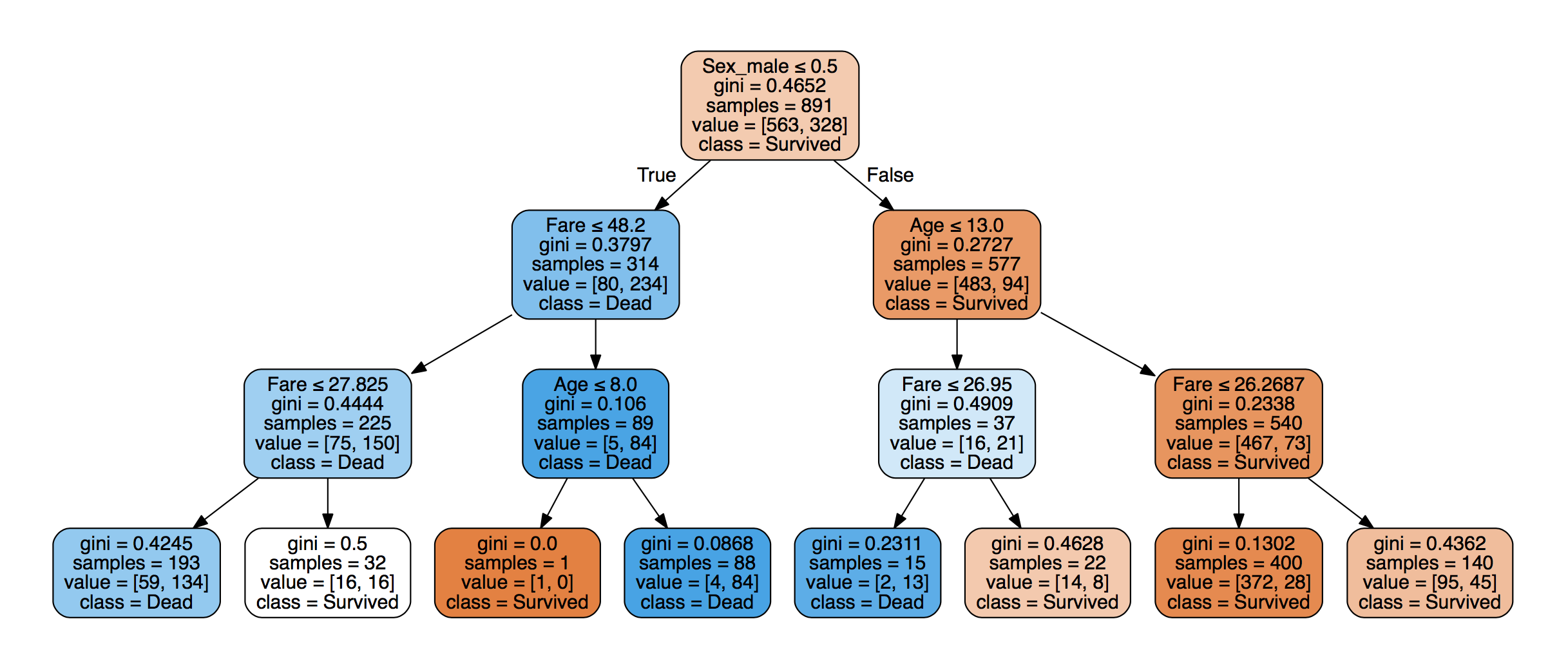
The maximal distance between the first decision and the last is 3, so that's max_depth=3.
Note: you can use graphviz to generate figures such as this. See the scikit-learn documentation here for further details.
In building this model, what you're essentially doing is creating a decision boundary in the space of feature variables, for example (image from here):

max_depth=3 ?The depth of the tree is known as a hyperparameter, which means a parameter you need to decide before you fit the model to the data. If you choose a larger max_depth, you'll get a more complex decision boundary.
If your decision boundary is too complex, you can overfit to the data, which means that your model will be describing noise as well as signal.
If your max_depth is too small, you might be underfitting the data, meaning that your model doesn't contain enough of the signal.
But how do you tell whether you're overfitting or underfitting?
Note: this is also referred to as the bias-variance trade-off; you won't go into details on that here, but we just mention it to be complete!
One way is to hold out a test set from your training data. You can then fit the model to your training data, make predictions on your test set and see how well your prediction does on the test set.
X_train, X_test, y_train, y_test = train_test_split(
    X, y, test_size=0.33, random_state=42, stratify=y)
max_depth ranging from 1 to 9 and plot the accuracy of the models on training and test sets:# Setup arrays to store train and test accuracies
dep = np.arange(1, 9)
train_accuracy = np.empty(len(dep))
test_accuracy = np.empty(len(dep))
# Loop over different values of k
for i, k in enumerate(dep):
# Setup a Decision Tree Classifier
clf = tree.DecisionTreeClassifier(max_depth=k)
# Fit the classifier to the training data
clf.fit(X_train, y_train)
#Compute accuracy on the training set
train_accuracy[i] = clf.score(X_train, y_train)
#Compute accuracy on the testing set
test_accuracy[i] = clf.score(X_test, y_test)
# Generate plot
plt.title('clf: Varying depth of tree')
plt.plot(dep, test_accuracy, label = 'Testing Accuracy')
plt.plot(dep, train_accuracy, label = 'Training Accuracy')
plt.legend()
plt.xlabel('Depth of tree')
plt.ylabel('Accuracy')
plt.show()
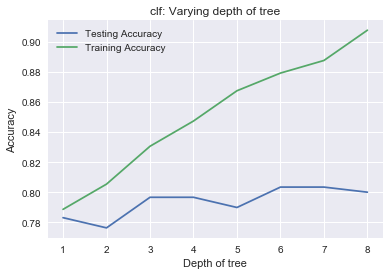
As you increase the max_depth, you're going to fit better and better to the training data because you'll make decisions that describe the training data. The accuracy for the training data will go up and up, but you see that this doesn't happen for the test data: you're overfitting.
So that's why you chose max_depth=3.
In this tutorial, you've got your data in a form to build first machine learning model. Nex,t you've built also your first machine learning model: a decision tree classifier. Lastly, you learned about train_test_split and how it helps us to choose ML model hyperparameters.
In the next tutorial, which will appear on the DataCamp Community on the 10th of January 2018, you'll learn how to engineer some new features and build some new models!
In the meantime, if you want to discover more on scikit-learn, check out DataCamp's Supervised Learning with scikit-learn course.
Machine Learning Courses
Course
Course
Tutorial
Avinash Navlani
Tutorial
Kurtis Pykes
Tutorial
Çağlar Uslu
Tutorial
Abid Ali Awan
Tutorial
Hugo Bowne-Anderson
code-along
George Boorman