ANOVA
If you have been analyzing ANOVA designs in traditional statistical packages, you are likely to find R's approach less coherent and user-friendly. A good online presentation on ANOVA in R can be found in ANOVA</a > section of the Personality Project. (Note: I have found that these pages render fine in Chrome and Safari browsers, but can appear distorted in iExplorer.)
1. Fit a Model
In the following examples lower case letters are numeric variables and upper case letters are factors.
# One Way Anova (Completely Randomized Design)
fit <- aov(y ~ A, data=mydataframe)
# Randomized Block Design (B is the blocking factor)
fit <- aov(y ~ A + B, data=mydataframe)# Two Way Factorial Design
fit <- aov(y ~ A + B + A:B, data=mydataframe)
fit <- aov(y ~ A*B, data=mydataframe)
# same thing# Analysis of Covariance
fit <- aov(y ~ A + x, data=mydataframe)For within subjects designs, the data frame has to be rearranged so that each measurement on a subject is a separate observation. See R and Analysis of Variance.
# One Within Factor
fit <- aov(y~A+Error(Subject/A),data=mydataframe)
# Two Within Factors W1 W2, Two Between Factors B1 B2
fit <- aov(y~(W1*W2*B1*B2)+Error(Subject/(W1*W2))+(B1*B2),
data=mydataframe)2. Look at Diagnostic Plots
Diagnostic plots provide checks for heteroscedasticity, normality, and influential observerations.```R layout(matrix(c(1,2,3,4),2,2)) # optional layout
plot(fit) # diagnostic plots
For details on the evaluation of test requirements, see [(M)ANOVA Assumptions](/stats/anovaAssumptions.html). ### 3. Evaluate Model Effects **WARNING** : R provides [Type I sequential SS](http://afni.nimh.nih.gov/sscc/gangc/SS.html), not the default [Type III marginal SS](http://afni.nimh.nih.gov/sscc/gangc/SS.html) reported by SAS and SPSS. In a nonorthogonal design with more than one term on the right hand side of the equation **order will matter** (i.e., A+B and B+A will produce _different_ results)! We will need use the **drop1( )** function to produce the familiar Type III results. It will compare each term with the full model. Alternatively, we can use anova(fit.model1, fit.model2) to compare nested models directly. ```R summary(fit) # display Type I ANOVA table drop1(fit,~.,test="F") # type III SS and F Tests
Nonparametric and resampling alternatives are available.
Multiple Comparisons
You can get Tukey HSD tests using the function below. By default, it calculates post hoc comparisons on each factor in the model. You can specify specific factors as an option. Again, remember that results are based on Type I SS!
# Tukey Honestly Significant Differences
TukeyHSD(fit) # where fit comes from aov()
Visualizing Results
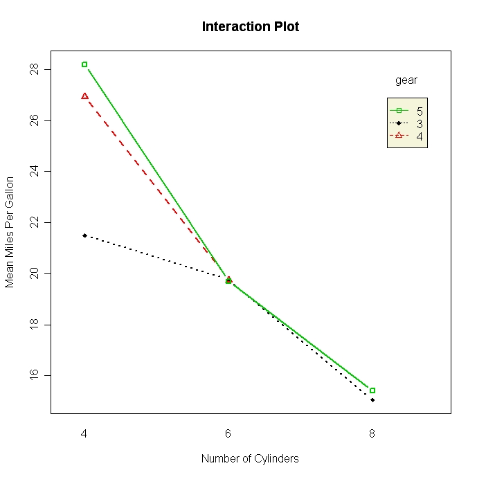
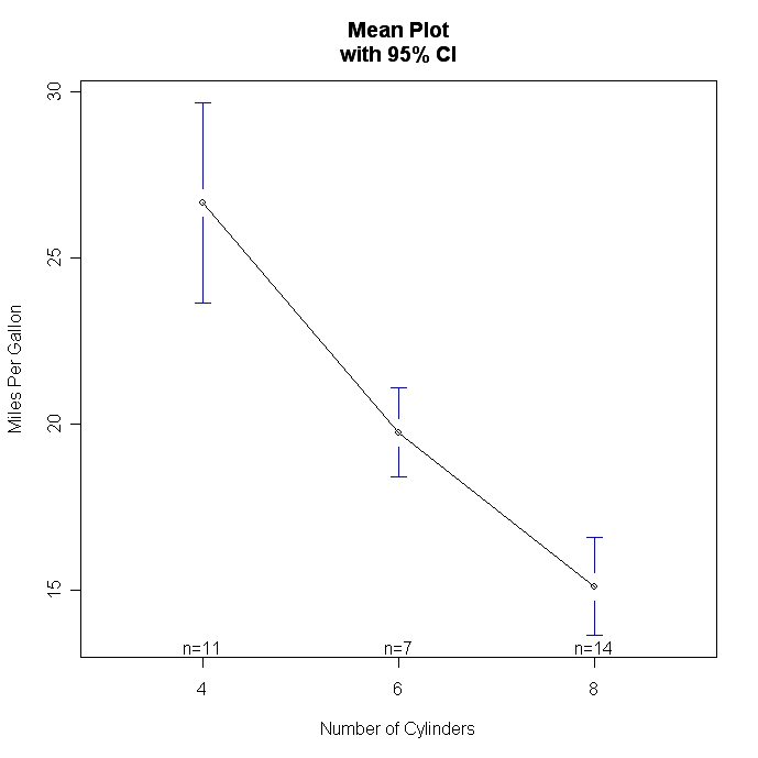
Use box plots and line plots to visualize group differences. There are also two functions specifically designed for visualizing mean differences in ANOVA layouts. interaction.plot( ) in the base stats package produces plots for two-way interactions. plotmeans( ) in the gplots</a >package produces mean plots for single factors, and includes confidence intervals.
# Two-way Interaction Plot
attach(mtcars)
gears <- factor(gears)
cyl <- factor(cyl)
interaction.plot(cyl, gear, mpg, type="b", col=c(1:3),
   leg.bty="o", leg.bg="beige", lwd=2, pch=c(18,24,22),
   xlab="Number of Cylinders",
   ylab="Mean Miles Per Gallon",
   main="Interaction Plot")
<
<
# Plot Means with Error Bars
library(gplots)
attach(mtcars)
cyl <- factor(cyl)
plotmeans(mpg~cyl,xlab="Number of Cylinders",
  ylab="Miles Per Gallon", main="Mean Plot\nwith 95% CI")
MANOVA
If there is more than one dependent (outcome) variable, you can test them simultaneously using a multivariate analysis of variance (MANOVA). In the following example, let Y be a matrix whose columns are the dependent variables.
# 2x2 Factorial MANOVA with 3 Dependent Variables.
Y <- cbind(y1,y2,y3)
fit <- manova(Y ~ A*B)
summary(fit, test="Pillai")
Other test options are "Wilks", "Hotelling-Lawley", and "Roy". Use summary.aov( ) to get univariate statistics. TukeyHSD( ) and plot( ) will not work with a MANOVA fit. Run each dependent variable separately to obtain them. Like ANOVA, MANOVA results in R are based on Type I SS. To obtain Type III SS, vary the order of variables in the model and rerun the analyses. For example, fit y~A*B for the TypeIII B effect and y~B*A for the Type III A effect.</span >
Going Further
R has excellent facilities for fitting linear and generalized linear mixed-effects models. The lastest implimentation is in package lme4. See the R News Article on Fitting Mixed Linear Models in R</a > for details.