LSTM Models: A Complete Guide to Long Short-Term Memory Networks

Standard recurrent neural networks struggle with memory. As sequences grow beyond 20-30 timesteps, gradients either shrink toward zero or blow up during backpropagation, and the network loses its ability to connect distant parts of the input. Hochreiter and Schmidhuber tackled this problem in their 1997 paper by introducing Long Short-Term Memory networks.

In this guide, I will walk through LSTM internals before moving to practical implementation in Python. The final sections compare LSTMs against Transformers so you can pick the right architecture for your use case.

I highly recommend our Introduction to Deep Learning in PyTorch course to get hands-on experience in using PyTorch to train neural networks, which are the basis for LSTM models.

What Is an LSTM Model?

LSTM stands for Long Short-Term Memory, a type of recurrent neural network (RNN) designed to handle sequences where context from much earlier in the input still matters.

The core idea behind LSTMs is a gating mechanism that regulates information flow through the network. Rather than letting all signals pass through equally, gates learn when to retain context and when to let it go. 

This selective memory allows LSTMs to track dependencies across hundreds of timesteps, which proved useful for language modeling, speech recognition, and time series forecasting. To understand why this architecture exists, it helps to see what breaks in standard RNNs.

The vanishing gradient problem in RNNs

Recurrent networks pass information from one timestep to the next through a hidden state. Each step multiplies this state by learned weights, updates it, and passes it forward. Training requires sending error signals backward through all those steps, and each backward pass shrinks the signal a bit. After enough steps, there's nothing left.

It's like making a photocopy of a photocopy. Do it a few times, and the copy looks fine. Do it fifty times, and you can barely read the text. RNNs hit this wall somewhere around 20-30 timesteps, which is why they struggle with longer sequences.

How LSTMs solve long-term dependencies

LSTMs add a separate memory track, called the cell state, that runs in parallel to the standard hidden state. The difference is structural: information in the cell state flows through addition rather than repeated multiplication, so it doesn't degrade the same way.

To control what goes into and out of this memory, LSTMs use gates. Each gate is a small neural network that learns to output values between 0 and 1, acting as a filter. A value near 0 blocks information; a value near 1 lets it through. The network learns during training which patterns are worth remembering across long sequences and which can be discarded.

This gating mechanism is what separates LSTMs from vanilla RNNs. Instead of forcing all information through the same path, LSTMs can selectively preserve context across hundreds of timesteps. The next section breaks down exactly how these gates work and how they combine to update the cell state.

LSTM model use cases

LSTMs appear wherever sequential data matters. A few examples beyond the usual NLP and forecasting applications:

• Banks run transaction sequences through LSTMs to catch fraud patterns that rule-based systems miss
• Hospitals monitor ECG streams with bidirectional LSTMs, catching cardiac anomalies faster than threshold alerts
• Smart city platforms predict traffic and energy demand from sensor feeds, adjusting resources before spikes hit
• Factories track equipment vibration over time to schedule maintenance before something breaks

LSTM Architecture: Gates and Memory Cells

This section covers LSTM internals in detail. If you want to jump straight to implementation, skip to the next section. The architecture details here aren't required to use LSTMs, but they help when debugging or tuning.

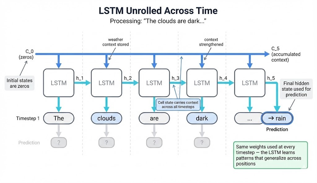
To understand how LSTMs work, we'll trace a concrete example: processing the sequence "The clouds are dark..." to predict the next word. Each component makes more sense when you can see what it does to actual data.

Cell state and hidden state in LSTMs

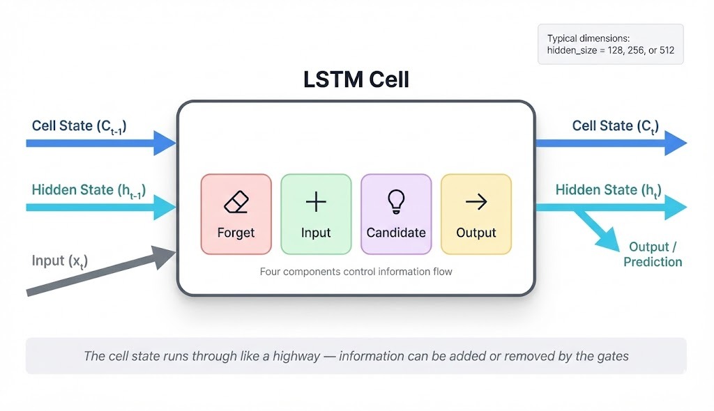
An LSTM maintains two separate vectors that flow through the network: the cell state and the hidden state.

The cell state acts as long-term storage. It carries information across timesteps with controlled modifications at each step. When processing our sequence, the cell state might store "weather-related noun appeared" after seeing "clouds" and preserve that context through "are", until "dark" reinforces the pattern.

The hidden state is the cell's output at each timestep. It feeds into predictions and into the next timestep's computations. After processing "dark," the hidden state encodes something like "adjective describing weather conditions" that a prediction layer can use.

Why two separate tracks? A single state would need to simultaneously hold long-term context and produce useful outputs. These goals conflict: stable memory requires minimal change, while useful outputs require transformation. Separating them lets each track optimize for its purpose.

At each timestep, the cell takes three inputs and produces two outputs:

Inputs:

• Previous cell state (C_{t-1}): what the network remembers so far

• Previous hidden state (h_{t-1}): the last timestep's output

• Current input (x_t): the new token, like "clouds" or "dark"

Outputs:

• Updated cell state (C_t): memory after processing this token

• New hidden state (h_t): this timestep's output

How LSTM gates compute

Four components control what happens inside the cell. Three of them are gates that output values between 0 and 1, acting as filters. The fourth is the candidate, who proposes new content.

When "are" arrives after "clouds," each component has a job:

• Forget gate (f_t): Should we keep the "clouds" context? Weather nouns followed by linking verbs usually matter, so the forget gate outputs values near 1 to preserve most of the cell state.

• Input gate (i_t): How much should "are" contribute to memory? Linking verbs carry less predictive signal, so the input gate outputs lower values.

• Candidate (C̃_t): What new information could "are" add? The candidate proposes content, but the input gate scales it down.

• Output gate (o_t): What should the hidden state show? The output gate filters the cell state to produce h_t.

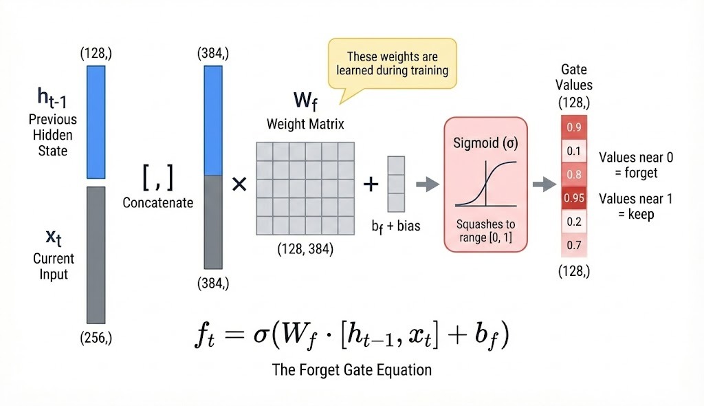
Each component computes its output the same way:

1. Concatenate h_{t-1} and x_t into one vector

2. Multiply by a learned weight matrix

3. Add a bias term

4. Apply an activation function

Gates use sigmoid activation, which squashes values to the 0-1 range. The candidate uses tanh, outputting values between -1 and 1, so it can propose both increases and decreases to the cell state.

The equations

Forget gate (sigmoid → 0 to 1):

Input gate (sigmoid → 0 to 1):

Output gate (sigmoid → 0 to 1):

Candidate (tanh → -1 to +1):

Each component has its own weight matrix (W_f, W_i, W_c, W_o), so they learn to respond to different patterns in the input.

How filtering works

Gate outputs multiply against vectors position-by-position (element-wise multiplication, written as ⊙). Each dimension gets filtered independently.

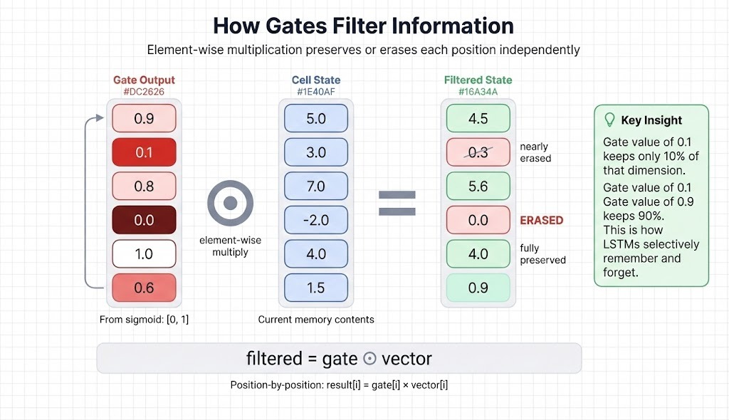
If a gate outputs 0.9 for position 1, that dimension keeps 90% of its value. If it outputs 0.0 for position 4, that dimension gets erased. When processing "dark" after "clouds are," the forget gate might output high values for dimensions storing noun/weather context and lower values for dimensions holding irrelevant earlier context.

Information flow between forget, add, and output gates

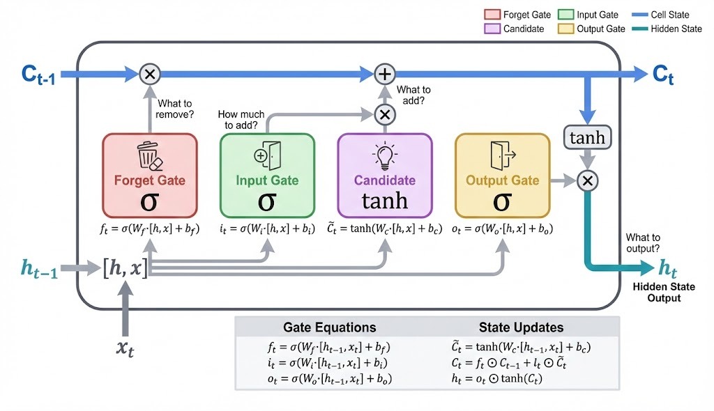
The components combine in three steps to update the cell state and produce the hidden state.

Step 1: Forget

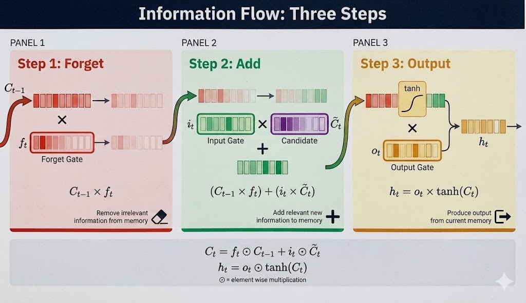
The forget gate filters the previous cell state:

Processing "dark," the forget gate preserves the weather context from "clouds" while clearing dimensions that tracked the article "The."

Step 2: Add

The input gate scales the candidate's proposal, then adds it to the filtered cell state:

The candidate might propose "adjective modifying weather noun," and the input gate decides how strongly to write that to memory. This additive update (not multiplicative) is what helps gradients flow during training.

Step 3: Output

The cell state passes through tanh, then the output gate filters what becomes the hidden state:

The tanh keeps values bounded. The output gate selects which aspects of the accumulated memory should be visible for predictions at this timestep.

The complete sequence:

Here's a simplified trace with a 4-dimensional cell state:

By timestep 4, dimensions 2-4 have accumulated a pattern. The hidden state h_4 feeds into a prediction layer (not part of the LSTM), which produces vocabulary probabilities. That accumulated pattern helps the model favor words like "rain" or "sky."

The network doesn't understand weather. It learns statistical correlations: certain input sequences tend to precede certain outputs.

Gradient flow during training

The cell state's additive structure provides a more direct gradient path than standard RNNs. If you're unfamiliar with how gradients propagate through neural networks, the backpropagation tutorial covers the fundamentals.

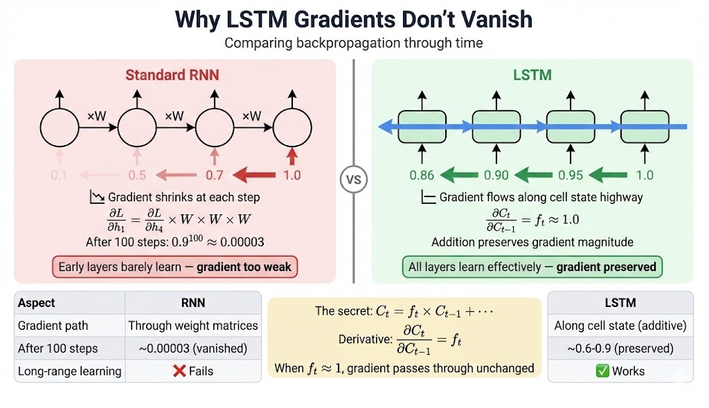
In standard RNNs, gradients flow through weight matrices at each step. Repeated multiplication compounds: after 100 steps with weights averaging 0.9, the gradient shrinks to 0.9^100 ≈ 0.00003.

LSTMs offer an alternative path along the cell state. The derivative of C_t with respect to C_{t-1}:

∂C_t/∂C_{t-1} = f_t

This is the forget gate value, not a weight matrix. When forget gates stay near 1, gradients pass through with less decay. If gates average 0.95, after 100 steps: 0.95^100 ≈ 0.006. Still reduced, but usable.

Practical note: Forget gate biases are often initialized to 1.0 or higher, pushing initial outputs toward "remember everything." This helps the network learn long-term patterns early in training.

LSTMs mitigate the vanishing gradient problem rather than eliminating it. The improvement comes from the additive cell-state update, which provides a gradient highway alongside the standard paths.

How to Implement LSTM Models in Python

The previous section covered what happens inside an LSTM cell: gates filtering information, cell state preserving context, and hidden state producing outputs. Now we'll see how PyTorch's nn.LSTM wraps all of that into a single module and uses it to classify movie reviews as positive or negative.

Tip for running the code: Training for 50 epochs on a CPU takes a long time. Use Google Colab or Kaggle Notebooks with GPU acceleration for faster results. The complete script is available as a GitHub Gist.

Building an LSTM Classifier with PyTorch

Text classification with LSTMs follows a pattern: convert words to vectors, let the LSTM process them sequentially, then use the final output for prediction.

Embedding words into vectors

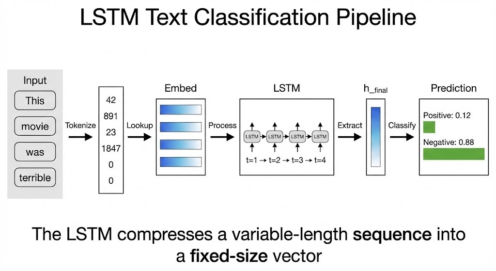
Neural networks operate on continuous numbers, but words are discrete symbols. We can't feed "terrible" directly into matrix multiplication. The solution is an embedding layer: a lookup table where each word maps to a learnable vector.

self.embedding = nn.Embedding(vocab_size, embedding_dim, padding_idx=padding_idx)

If you choose embedding_dim=32, every word becomes a 32-dimensional vector. Early in training, these vectors are random. As the model learns, words with similar sentiment drift closer together in this vector space. "Terrible," "awful," and "boring" might end up near each other, while "excellent" and "amazing" cluster elsewhere.

The padding_idx argument tells the layer to keep padding tokens at zero vectors, so they don't influence the model.

Defining the LSTM architecture

self.lstm = nn.LSTM(
	input_size=embedding_dim,
	hidden_size=hidden_size,
	num_layers=num_layers,
	batch_first=True,
	dropout=dropout if num_layers > 1 else 0,
	bidirectional=bidirectional,
)

This single line creates the entire gate machinery from the previous section. The hidden_size determines how much information the cell state and hidden state can carry. Larger values let the model track more patterns but require more computation.

Setting batch_first=True means inputs are shaped (batch, sequence_length, embedding_dim). The LSTM processes each position left to right, updating its internal states at each step.

Processing the sequence

After processing "This movie was absolutely terrible," the LSTM has seen every word. Its final hidden state has accumulated whatever the model learned to extract from that sequence. For sentiment, this might encode something like "strong negative adjective at the end, negating earlier neutral content."

def forward(self, x):
	embedded = self.embedding(x)
	lstm_out, (h_n, c_n) = self.lstm(embedded)
	h_final = h_n[-1]
	return self.fc(h_final)

The LSTM returns both per-timestep outputs (lstm_out) and final states (h_n, c_n). For classification, we only need h_n[-1], the hidden state after the last token. A linear layer then maps this to class scores.

Tracing a review through the model

When "This movie was terrible" enters the classifier:

1. Each word gets its embedding: four vectors of shape (32,)

2. The LSTM processes them sequentially. "This" initializes some cell state. "Movie" updates it slightly. "Was" is neutral and changes little. "Terrible" triggers the forget gate to clear irrelevant context and the input gate to write a strong negative signal.

3. The final hidden state captures the accumulated pattern.

4. The linear layer maps this to two scores: one for positive, one for negative

The model doesn't understand language. It learns statistical patterns: certain word sequences correlate with certain labels.

The full model class

Below, you can see the whole LSTMClassifier class we just created step-by-step:

import torch
import torch.nn as nn
from torch.utils.data import DataLoader, TensorDataset
from datasets import load_dataset
from collections import Counter
import numpy as np
 
torch.manual_seed(42)
np.random.seed(42)
 
 
class LSTMClassifier(nn.Module):
    def __init__(
        Self,
        Vocab_size,
        Embedding_dim,
        Hidden_size,
        Output_size,
        num_layers=1,
        dropout=0.0,
        bidirectional=False,
        padding_idx=0,
    ):
        super().__init__()
        self.hidden_size = hidden_size
    	self.num_layers = num_layers
    	self.bidirectional = bidirectional
 
    	self.embedding = nn.Embedding(
	    vocab_size, embedding_dim, padding_idx=padding_idx
        )
    	self.lstm = nn.LSTM(
            input_size=embedding_dim,
            hidden_size=hidden_size,
            num_layers=num_layers,
            batch_first=True,
            dropout=dropout if num_layers > 1 else 0,
            bidirectional=bidirectional,
    	)	
 
    	fc_input_size = hidden_size * 2 if bidirectional else hidden_size
    	self.fc = nn.Linear(fc_input_size, output_size)
 
    def forward(self, x):
    	embedded = self.embedding(x)
    	lstm_out, (h_n, c_n) = self.lstm(embedded)
 
    	if self.bidirectional:
            h_final = torch.cat([h_n[-2], h_n[-1]], dim=1)
    	else:
            h_final = h_n[-1]
 
    	return self.fc(h_final)

The bidirectional option runs two LSTMs: one left-to-right, one right-to-left. Their final hidden states are concatenated, providing the model with context from both directions. This helps when meaning depends on what comes after, like "not bad," where "not" only makes sense given "bad."

Preparing text for the model

LSTMs need integer sequences, not strings. Preprocessing converts raw text through three steps: 

1. Build a vocabulary mapping words to indices
2. Convert each review to a sequence of indices
3. Pad sequences to uniform length

def build_vocab(texts, max_vocab_size=10000):
	counter = Counter()
	for text in texts:
    		counter.update(text.lower().split())
 
	vocab = {"<pad>": 0, "<unk>": 1}
	for word, _ in counter.most_common(max_vocab_size - 2):
    		vocab[word] = len(vocab)
	return vocab

We reserve index 0 for padding and index 1 for unknown words. Limiting vocabulary size filters rare words that lack enough examples to learn meaningful embeddings.

def tokenize_and_pad(texts, vocab, max_length=200):
	sequences = []
	for text in texts:
    		tokens = text.lower().split()
    		ids = [vocab.get(t, vocab["<unk>"]) for t in tokens[:max_length]]
    		ids = ids + [vocab["<pad>"]] * (max_length - len(ids))
    		sequences.append(ids)
	return torch.tensor(sequences, dtype=torch.long)

Truncating to max_length limits how far back the LSTM must remember. Longer sequences preserve more context but increase computational and memory costs. For movie reviews, 100-200 tokens usually capture the key sentiment signals.

Padding ensures that every sequence has the same length, allowing PyTorch to batch them into a single tensor. The padding tokens become zero vectors after embedding and contribute little to the final state.

def load_imdb_data(max_samples=10000, max_length=200, max_vocab=10000):
	dataset = load_dataset("imdb")
 
	train_data = dataset["train"].shuffle(seed=42)
	test_data = dataset["test"].shuffle(seed=42)
 
	train_texts = train_data["text"][:max_samples]
	train_labels = train_data["label"][:max_samples]
	test_texts = test_data["text"][: max_samples // 4]
	test_labels = test_data["label"][: max_samples // 4]
 
	vocab = build_vocab(train_texts, max_vocab)
 
	X_train = tokenize_and_pad(train_texts, vocab, max_length)
	X_test = tokenize_and_pad(test_texts, vocab, max_length)
	y_train = torch.tensor(train_labels, dtype=torch.long)
	y_test = torch.tensor(test_labels, dtype=torch.long)
 
	return X_train, y_train, X_test, y_test, vocab

Building vocabulary only from training data prevents information leakage. If a rare word appears only in test reviews, the model should treat it as unknown rather than having learned its embedding during training.

LSTM training and hyperparameters

The training loop updates the model's weights based on how far its predictions are from the correct values. For LSTMs, one detail matters more than usual: gradient clipping.

def train_model(model, train_loader, test_loader, n_epochs=5, lr=0.001):
	criterion = nn.CrossEntropyLoss()
	optimizer = torch.optim.Adam(model.parameters(), lr=lr)
 
	for epoch in range(n_epochs):
    		model.train()
    		total_loss, correct, total = 0, 0, 0
 
    		for batch_texts, batch_labels in train_loader:
        		optimizer.zero_grad()
        		outputs = model(batch_texts)
        		loss = criterion(outputs, batch_labels)
        		loss.backward()
            		torch.nn.utils.clip_grad_norm_(
	model.parameters(), 
	max_norm=5.0)
        		optimizer.step()
 
        		total_loss += loss.item()
        		_, predicted = outputs.max(1)
        		correct += (predicted == batch_labels).sum().item()
        		total += batch_labels.size(0)

Why gradient clipping matters for LSTMs

Earlier, we explained how LSTMs mitigate vanishing gradients through additive updates to the cell state. But exploding gradients remain a risk. When gradients grow too large, weight updates overshoot and destabilize training.

clip_grad_norm_ caps the total gradient magnitude. If gradients would exceed max_norm=5.0, they get scaled down proportionally. This keeps updates stable without eliminating the gradient signal entirely.

    	model.eval()
    	test_correct, test_total = 0, 0
    	with torch.no_grad():
        	for batch_texts, batch_labels in test_loader:
            		outputs = model(batch_texts)
            		_, predicted = outputs.max(1)
            		test_correct += (predicted == batch_labels).sum().item()
            		test_total += batch_labels.size(0)
 
    	test_acc = test_correct / test_total
    	print(f"Epoch {epoch+1}: Loss={total_loss/len(train_loader):.4f}, "
          	f"Train={correct/total:.3f}, Test={test_acc:.3f}")
 
    return test_acc

model.eval() disables dropout during evaluation. torch.no_grad() skips gradient computation since we're not updating weights, which saves memory and speeds up inference.

Choosing hyperparameters

X_train, y_train, X_test, y_test, vocab = load_imdb_data(
	max_samples=10000, max_length=100, max_vocab=5000
)
 
train_loader = DataLoader(TensorDataset(X_train, y_train), batch_size=64, shuffle=True)
test_loader = DataLoader(TensorDataset(X_test, y_test), batch_size=64)
 
model = LSTMClassifier(
	vocab_size=len(vocab),
	embedding_dim=32,
	hidden_size=32,
	output_size=2,
	padding_idx=vocab["<pad>"],
)
 
final_acc = train_model(model, train_loader, test_loader, n_epochs=50, lr=0.001)

These values reflect tradeoffs:

• hidden_size=32: Small enough for fast iteration. Production models often use 128-512, but with increasing size, gains diminish and training slows down.

• embedding_dim=32: Matching hidden size is common but not required. Larger embeddings capture finer word distinctions at the cost of more parameters.

• max_length=100: Most sentiment signals appear early in reviews. Longer sequences help with nuanced cases, but quadruple memory usage for a double-long max_length.

• batch_size=64: Larger batches give more stable gradient estimates. Smaller batches can help escape local minima. 32-128 is typical.

• lr=0.001: Adam's default works for most LSTM tasks. If loss oscillates, try 0.0001. If learning stalls, try 0.01.

• n_epochs=50: Enough for the model to converge. Watch for test accuracy plateauing or dropping while train accuracy keeps climbing, which signals overfitting.

What the model learns

Running this configuration produces output like:

...
Epoch 46: Loss=0.4126, Train=0.812, Test=0.789
Epoch 47: Loss=0.4054, Train=0.815, Test=0.791
Epoch 48: Loss=0.3998, Train=0.818, Test=0.788
Epoch 49: Loss=0.3921, Train=0.821, Test=0.793
Epoch 50: Loss=0.3867, Train=0.824, Test=0.795

Training accuracy reaches around 82% while test accuracy settles near 80%. The model learns which word patterns predict sentiment. Strong adjectives near the end carry weight. Negations like "not" flip polarity. Certain phrases ("waste of time," "highly recommend") become strong signals. None of this is programmed; it emerges from correlations in the training data.

With minimal tuning and a small model, 80% accuracy is reasonable. The small gap between training and test accuracy shows the model generalizes well without severe overfitting. Adding dropout, using pretrained embeddings like GloVe, or training on more data would push accuracy into the high 80s.

Improving LSTM Model Performance

The basic LSTM architecture from the previous sections works, but several techniques can push accuracy higher without switching to a different model family. These approaches have been validated across thousands of production deployments and research papers.

Bidirectional LSTMs

Standard LSTMs process sequences left-to-right, building context from past tokens only. Bidirectional LSTMs (BiLSTMs) run two parallel passes: one forward, one backward. The final representation at each timestep combines what came before and what comes after.

self.lstm = nn.LSTM(
	input_size=embedding_dim,
	hidden_size=hidden_size,
	bidirectional=True,  # Run both directions
	batch_first=True,
)
# Output size doubles: hidden_size * 2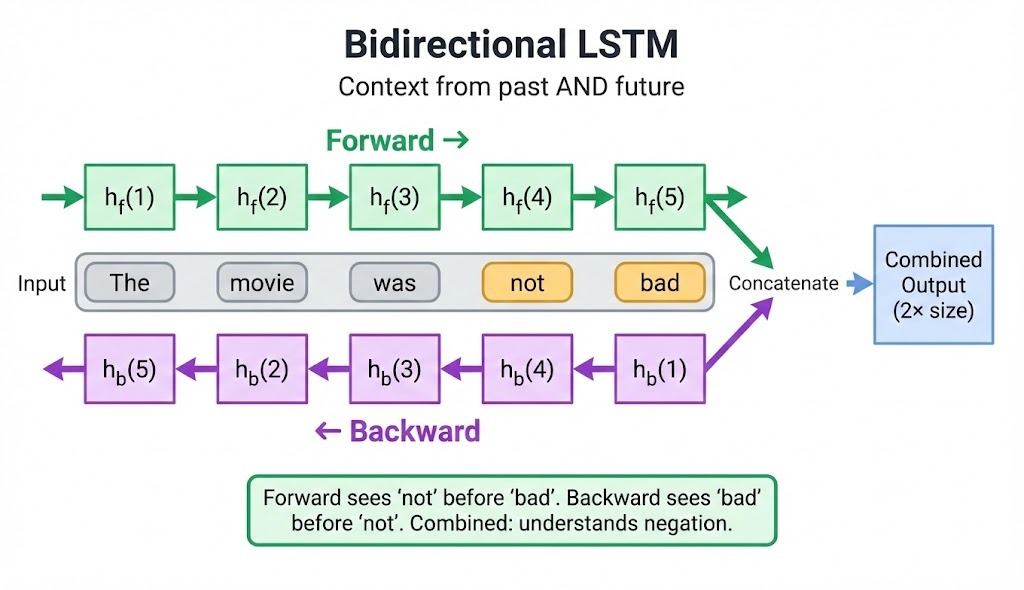

For sentiment analysis, this matters when negation appears after the word it modifies: "the movie was not bad" needs forward context to know "bad" exists, and backward context to know "not" precedes it. 

BiLSTMs consistently outperform unidirectional models on named entity recognition (NER), sentiment classification, and speech recognition, with typical gains of 5-15%.

The tradeoff: you need the full sequence at inference time. Streaming applications that receive tokens one by one can't use bidirectional processing.

Adding attention

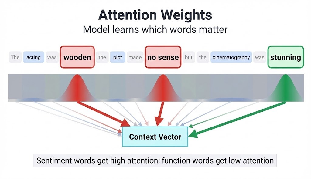
Attention lets the model weight which timesteps matter most for a given prediction. Instead of compressing an entire sequence into a single final hidden state, attention computes a weighted combination of all hidden states.

class AttentionLayer(nn.Module):
	def __init__(self, hidden_size):
    		super().__init__()
    		self.attention = nn.Linear(hidden_size, 1)
	
	def forward(self, lstm_outputs):
    	# lstm_outputs: (batch, seq_len, hidden_size)
    		scores = self.attention(lstm_outputs)  # (batch, seq_len, 1)
    		weights = torch.softmax(scores, dim=1)
    		context = torch.sum(weights * lstm_outputs, dim=1)
    		return context

In a review like "The acting was wooden, the plot made no sense, but the cinematography was stunning," attention learns to focus on sentiment-bearing phrases rather than treating all words equally. The model assigns higher weights to "wooden," "no sense," and "stunning" while downweighting "the" and "was."

Attention adds minimal computational overhead and often yields 2-5% accuracy improvements on classification tasks. For sequence-to-sequence problems like translation, attention between the encoder and decoder is nearly mandatory for good performance.

Stacking LSTM layers

A single LSTM layer captures patterns at one level of abstraction. Stacking multiple layers lets the network learn hierarchical features: the first layer might detect local phrase patterns, while higher layers combine these into document-level understanding.

self.lstm = nn.LSTM(
	input_size=embedding_dim,
	hidden_size=hidden_size,
	num_layers=3,  # Stack three layers
	dropout=0.3,   # Dropout between layers (not within)
	batch_first=True,
)

Guidelines for depth:

•  1 layer: Simple tasks, small datasets, fast iteration
• 2 layers: Most production applications
• 3-4 layers: Complex temporal dependencies, large datasets
• Beyond 4: Diminishing returns, training instability

Each additional layer roughly doubles training time. Start shallow and add depth only if validation metrics plateau.

Regularization techniques

LSTMs overfit easily, especially on small datasets. Three regularization techniques work well together:

• Dropout
• Gradient clipping
• Early stopping

Dropout

Dropout randomly zeros neurons during training, forcing the network to distribute learning across multiple pathways. Apply dropout between LSTM layers, not inside the recurrent connections (which can disrupt temporal learning).

# PyTorch applies dropout between stacked layers automatically
self.lstm = nn.LSTM(..., num_layers=2, dropout=0.3)
 
# For single-layer LSTMs, add dropout after
self.dropout = nn.Dropout(0.3)

Dropout rates of 0.2-0.5 work for most tasks. Higher values help with severe overfitting but slow convergence.

Gradient clipping

Gradient clipping caps the magnitudes of gradients during backpropagation. While LSTMs mitigate vanishing gradients, exploding gradients still occur, especially with long sequences or deep networks.

torch.nn.utils.clip_grad_norm_(model.parameters(), max_norm=5.0)

Values between 1.0 and 5.0 are typical. If training loss spikes or produces NaN values, lower the threshold.

Early stopping

Early stopping monitors validation loss and halts training when it stops improving. This prevents the model from memorizing training data at the expense of generalization.

patience = 5
best_val_loss = float('inf')
epochs_without_improvement = 0
 
for epoch in range(max_epochs):
	train_loss = train_one_epoch(model, train_loader)
	val_loss = evaluate(model, val_loader)
	
	if val_loss < best_val_loss:
    		best_val_loss = val_loss
    		epochs_without_improvement = 0
    		torch.save(model.state_dict(), 'best_model.pt')
	else:
    		epochs_without_improvement += 1
	if epochs_without_improvement >= patience:
        	break

For a complete walkthrough of training loops, evaluation metrics, and debugging common issues in LSTMs, see the NLP with PyTorch guide.

Pretrained embeddings

Random embedding initialization works, but pretrained embeddings like GloVe or Word2Vec give the model a head start. These embeddings encode semantic relationships learned from billions of words: "king" and "queen" end up near each other, as do "terrible" and "awful."

import numpy as np
 
def load_glove_embeddings(glove_path, vocab, embedding_dim):
	embeddings = np.random.randn(len(vocab), embedding_dim) * 0.01
	
	with open(glove_path, 'r') as f:
    	for line in f:
        	parts = line.split()
        	word = parts[0]
        	if word in vocab:
            		embeddings[vocab[word]] = np.array(parts[1:], dtype=np.float32)
	
	return torch.tensor(embeddings, dtype=torch.float32)
 
# Load and freeze or fine-tune
pretrained = load_glove_embeddings('glove.6B.100d.txt', vocab, 100)
model.embedding.weight.data.copy_(pretrained)
model.embedding.weight.requires_grad = True  # Fine-tune during training

Pretrained embeddings help most when training data is limited. With millions of examples, randomly initialized embeddings eventually catch up. For most practical applications with 10k-100k samples, expect 3-8% accuracy gains from pretrained initialization.

Combining techniques

These approaches stack. A production-grade text classifier might use:

• BiLSTM for bidirectional context
• 2 stacked layers for hierarchical features
• Attention pooling instead of the final hidden state
• GloVe embeddings fine-tuned during training
• Dropout of 0.3 between layers
• Gradient clipping at 5.0
• Early stopping with patience of 5 epochs

Each addition increases complexity and training time. Start with a baseline single-layer LSTM, measure performance, then add techniques one at a time to see what provides gains on your specific task.

LSTM vs Transformers: Choosing the Right Architecture

LSTMs ran the show for sequence modeling from the late 1990s through the mid-2010s. The 2017 "Attention Is All You Need" paper changed that. Transformers now power most large language models, but LSTMs haven't disappeared. They fill different niches.

LSTM limitations

Earlier sections covered how LSTMs process sequences one token at a time and why that gating mechanism works. At scale, that sequential dependency becomes a bottleneck. Your GPU might have thousands of cores, but most sit idle while the hidden state chain finishes. A 500-token input means 500 operations in a row.

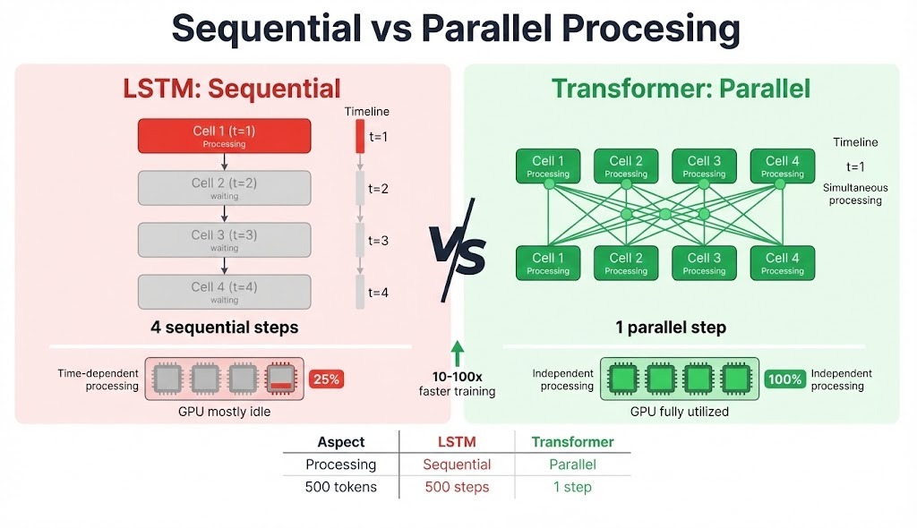
Transformers don't have this constraint. Self-attention computes relationships between all positions simultaneously, so the same 500-token sequence is processed in parallel. On modern hardware with large batch sizes, this translates to 10-100x training speedups.

The sequence length ceiling matters too. We saw how LSTMs preserve gradients better than vanilla RNNs, but "better" doesn’t mean "perfect." Performance still drops somewhere around 200-500 tokens, depending on the task. 

Transformers compute attention between every pair of positions directly, so token 1 attends to token 1000 with equal ease. The tradeoff is memory: attention matrices grow quadratically with sequence length.

Gate activations also make interpretation difficult. Values range from 0 to 1 without clear boundaries. Attention weights in Transformers aren't perfect explanations either, but they give a clearer signal about which input tokens mattered for each output.

When to use LSTM vs transformers

Transformers make sense when:

• Training data exceeds 100K examples, and you have GPU access
• The task involves dependencies spanning hundreds of tokens
• Training speed matters for iteration cycles
• Pretrained models like GPT can be fine-tuned for your use case

LSTMs still fit when:

• The target device has tight memory constraints (edge, embedded, mobile)
• Data is scarce (under 10K examples), and Transformer overfitting becomes a concern
• Predictions need to happen on partial sequences before the full input arrives
• Latency budgets demand lightweight models

Time series forecasting lands somewhere in the middle. Recent benchmarks show that both architectures perform similarly on univariate data, with consistent patterns. Transformers pull ahead when multiple features interact in complex ways, but LSTMs hold up when data is scarce or compute is tight.

Hybrid designs blend the two approaches. Some architectures stack LSTM layers with attention mechanisms. xLSTM, published in 2024, revisits the original design with exponential gating and matrix memory, showing competitive results with Transformers at smaller scales.

The decision usually comes down to constraints. Unlimited compute and data? Transformers win on most NLP tasks. A microcontroller with 10K training examples? LSTMs remain practical.

Conclusion

LSTMs solved a real problem when they arrived in 1997. The gating mechanism introduced by Hochreiter and Schmidhuber enabled networks to finally learn from sequences longer than a few dozen tokens. That architecture powered machine translation, speech recognition, and time series forecasting for nearly two decades.

Transformers now handle most large-scale NLP tasks, but LSTMs haven't become obsolete. They still make sense for edge deployment, streaming applications, and situations where training data is limited.

If you're starting a new sequence modeling project, try a simple LSTM first. Measure its performance, understand its failure modes, then decide whether the problem actually requires a Transformer. The concepts from this guide (gating, cell state, gradient flow) transfer directly to understanding more complex architectures.

For hands-on practice, I recommend taking our Recurrent Neural Networks course, which walks through additional LSTM applications with guided exercises.