Course
In this tutorial, you will learn how to use a time-series model called Long Short-Term Memory. LSTM models are powerful, especially for retaining long-term memory, by design, as you will see later. You'll tackle the following topics in this tutorial:
- Understand why you would need to be able to predict stock price movements.
- Download the data - You will use stock market data from Yahoo Finance.
- Split train-test data and also perform some data normalization.
- Go over and apply a few averaging techniques that can be used for one-step-ahead predictions.
- Motivate and briefly discuss an LSTM model as it allows one to predict more than one step ahead.
- Predict and visualize future stock market with current data
If you're unfamiliar with deep learning or neural networks, you should look at our Deep Learning in Python course. It covers the basics, as well as how to build a neural network on your own in Keras. This package is different from TensorFlow, which will be used in this tutorial, but the idea is the same.
Why Do You Need Time Series Models?
You would like to model stock prices correctly so as a stock buyer, you can reasonably decide when to buy stocks and when to sell them to make a profit. This is where time series modeling comes in. You need good machine learning models that can look at the history of a sequence of data and correctly predict what the future elements of the sequence are going to be.
Warning: Stock market prices are highly unpredictable and volatile. This means that no consistent patterns in the data allow you to model stock prices over time near-perfectly. Don't take it from me; take it from Princeton University economist Burton Malkiel, who argues in his 1973 book, "A Random Walk Down Wall Street," that if the market is truly efficient and a share price reflects all factors immediately as soon as they're made public, a blindfolded monkey throwing darts at a newspaper stock listing should do as well as any investment professional.
However, let's not go all the way believing that this is just a stochastic or random process and that there is no hope for machine learning. Let's see if you can at least model the data so that the predictions you make correlate with the actual behavior of the data. In other words, you don't need the exact stock values of the future but the stock price movements (that is, if it is going to rise or fall in the near future).
# Make sure that you have all these libaries available to run the code successfully
from pandas_datareader import data
import matplotlib.pyplot as plt
import pandas as pd
import datetime as dt
import urllib.request, json
import os
import numpy as np
import tensorflow as tf # This code has been tested with TensorFlow 1.6
from sklearn.preprocessing import MinMaxScaler
Downloading the Data
You will be using data from the following sources:
-
Alpha Vantage Stock API. Before you start, however, you will first need an API key, which you can obtain for free here. After that, you can assign that key to the
api_keyvariable. This tutorial will retrieve 20 years of historical data for the American Airlines stock. As an optional reading, you may refer to this stock API starter guide for the best practices for working with historical market data. -
Use the data from this page. Copy the Stocks folder in the zip file to your project home folder.
Stock prices come in several different flavors. They are,
- Open: Opening stock price of the day
- Close: Closing stock price of the day
- High: Highest stock price of the data
- Low: Lowest stock price of the day
Getting data from Alpha Vantage
You will first load the data from Alpha Vantage. Since you're going to make use of the American Airlines stock market prices to make your predictions, you set the ticker to "AAL". Additionally, you also define a url_string, which will return a JSON file with all the stock market data for American Airlines within the last 20 years, and a file_to_save, which will be the file to which you save the data. You'll use the ticker variable that you defined beforehand to help name this file.
Next, you're going to specify a condition: if you haven't already saved data, you will go ahead and grab the data from the URL that you set in url_string; You'll store the date, low, high, volume, close, open values to a pandas DataFrame df and you'll save it to file_to_save. However, if the data is already there, you'll just load it from the CSV.
Getting data from Kaggle
The data found on Kaggle is a collection of CSV files, and you don't have to do any preprocessing, so you can directly load the data into a Pandas DataFrame.
data_source = 'kaggle' # alphavantage or kaggle

if data_source == 'alphavantage':
    # ====================== Loading Data from Alpha Vantage ==================================

    api_key = '<your API key>'

    # American Airlines stock market prices
    ticker = "AAL"

    # JSON file with all the stock market data for AAL from the last 20 years
    url_string = "https://www.alphavantage.co/query?function=TIME_SERIES_DAILY&symbol=%s&outputsize=full&apikey=%s"%(ticker,api_key)

    # Save data to this file
    file_to_save = 'stock_market_data-%s.csv'%ticker

    # If you haven't already saved data,
    # Go ahead and grab the data from the url
    # And store date, low, high, volume, close, open values to a Pandas DataFrame
    if not os.path.exists(file_to_save):
        with urllib.request.urlopen(url_string) as url:
            data = json.loads(url.read().decode())
            # extract stock market data
            data = data['Time Series (Daily)']
            df = pd.DataFrame(columns=['Date','Low','High','Close','Open'])
            for k,v in data.items():
                date = dt.datetime.strptime(k, '%Y-%m-%d')
                data_row = [date.date(),float(v['3. low']),float(v['2. high']),
                            float(v['4. close']),float(v['1. open'])]
                df.loc[-1,:] = data_row
                df.index = df.index + 1
        print('Data saved to : %s'%file_to_save)
        df.to_csv(file_to_save)

    # If the data is already there, just load it from the CSV
    else:
        print('File already exists. Loading data from CSV')
        df = pd.read_csv(file_to_save)

else:

    # ====================== Loading Data from Kaggle ==================================
    # You will be using HP's data. Feel free to experiment with other data.
    # But while doing so, be careful to have a large enough dataset and also pay attention to the data normalization
    df = pd.read_csv(os.path.join('Stocks','hpq.us.txt'),delimiter=',',usecols=['Date','Open','High','Low','Close'])
    print('Loaded data from the Kaggle repository')
Data saved to : stock_market_data-AAL.csv
Data exploration
Here, you will print the data you collected into the DataFrame. You should also make sure that the data is sorted by date because the order of the data is crucial in time series modeling.
# Sort DataFrame by date
df = df.sort_values('Date')

# Double check the result
df.head()
| Date | Open | High | Low | Close | |
|---|---|---|---|---|---|
| 0 | 1970-01-02 | 0.30627 | 0.30627 | 0.30627 | 0.30627 |
| 1 | 1970-01-05 | 0.30627 | 0.31768 | 0.30627 | 0.31385 |
| 2 | 1970-01-06 | 0.31385 | 0.31385 | 0.30996 | 0.30996 |
| 3 | 1970-01-07 | 0.31385 | 0.31385 | 0.31385 | 0.31385 |
| 4 | 1970-01-08 | 0.31385 | 0.31768 | 0.31385 | 0.31385 |
Data visualization
Now, let's see what sort of data you have. You want data with various patterns occurring over time.
plt.figure(figsize = (18,9))
plt.plot(range(df.shape[0]),(df['Low']+df['High'])/2.0)
plt.xticks(range(0,df.shape[0],500),df['Date'].loc[::500],rotation=45)
plt.xlabel('Date',fontsize=18)
plt.ylabel('Mid Price',fontsize=18)
plt.show()
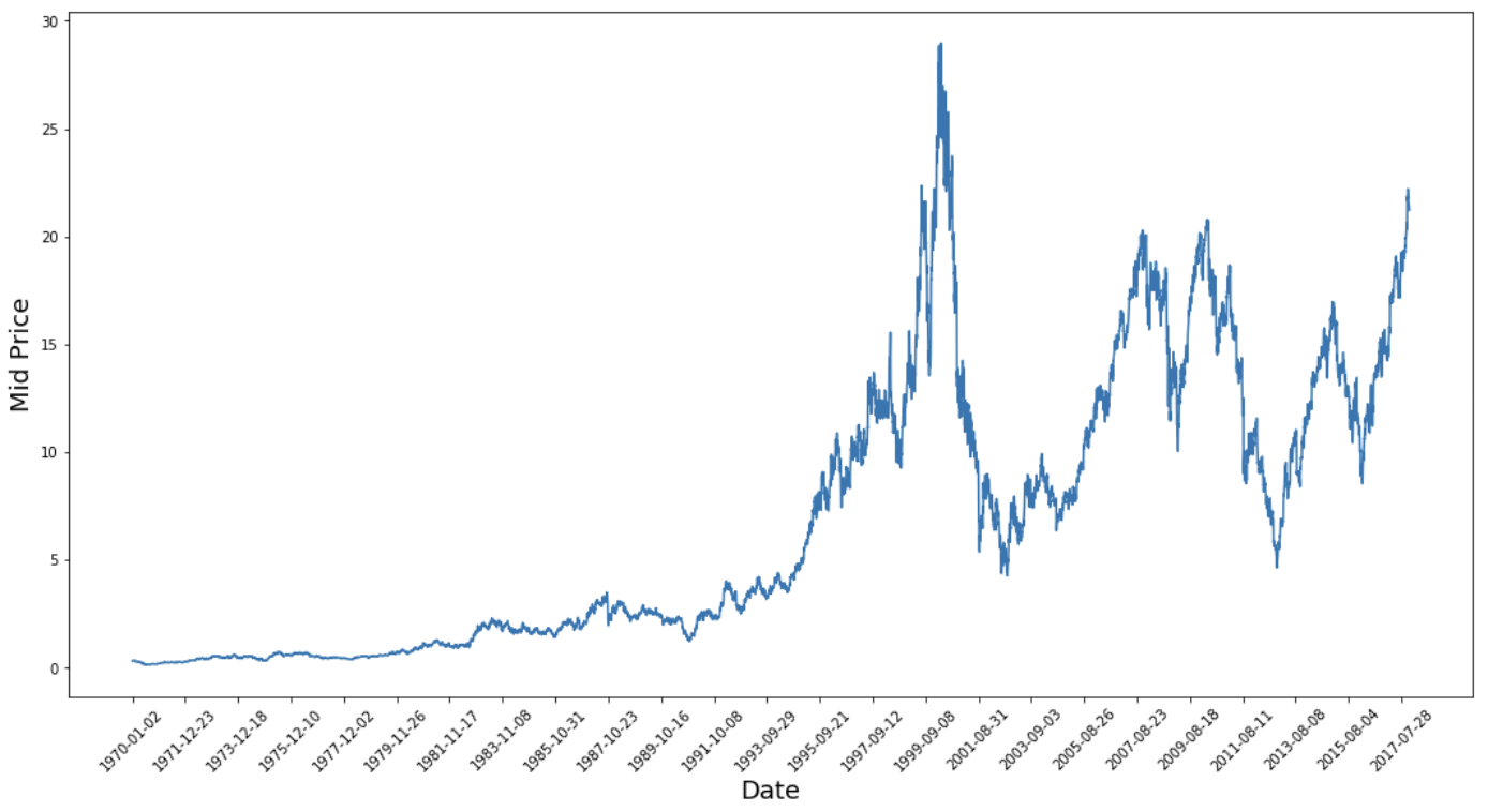
This graph already says a lot. The specific reason I picked this company over others is that it is bursting with different stock price behaviors over time. This will make the learning more robust and give you a chance to test how good the predictions are for a variety of situations.
Another thing to notice is that the values close to 2017 are much higher and fluctuate more than those close to the 1970s. Therefore, you need to ensure that the data behaves in similar value ranges throughout the time frame. You will take care of this during the data normalization phase.
Become an ML Scientist
Splitting Data Into a Training Set and a Test Set
You will use the mid-price, which is calculated by taking the average of the highest and lowest recorded prices on a day.
# First calculate the mid prices from the highest and lowest
high_prices = df.loc[:,'High'].as_matrix()
low_prices = df.loc[:,'Low'].as_matrix()
mid_prices = (high_prices+low_prices)/2.0
Now, you can split the training data and test data. The training data will be the first 11,000 data points of the time series, and the rest will be test data.
train_data = mid_prices[:11000]
test_data = mid_prices[11000:]
Normalizing the Data
Now, you need to define a scaler to normalize the data. MinMaxScalar scales all the data to be in the region of 0 and 1. You can also reshape the training and test data to be in the shape [data_size, num_features].
# Scale the data to be between 0 and 1
# When scaling remember! You normalize both test and train data with respect to training data
# Because you are not supposed to have access to test data
scaler = MinMaxScaler()
train_data = train_data.reshape(-1,1)
test_data = test_data.reshape(-1,1)
Due to your earlier observation that different time periods of data have different value ranges, you normalize the data by splitting the full series into windows. If you don't do this, the earlier data will be close to 0 and will not add much value to the learning process. Here, you choose a window size of 2500.
Tip: When choosing the window size, make sure it's not too small. When you perform windowed normalization, it can introduce a break at the very end of each window, as each window is normalized independently.
In this example, 4 data points will be affected by this. But given you have 11,000 data points, 4 points will not cause any issue.
# Train the Scaler with training data and smooth data
smoothing_window_size = 2500
for di in range(0,10000,smoothing_window_size):
    scaler.fit(train_data[di:di+smoothing_window_size,:])
    train_data[di:di+smoothing_window_size,:] = scaler.transform(train_data[di:di+smoothing_window_size,:])

# You normalize the last bit of remaining data
scaler.fit(train_data[di+smoothing_window_size:,:])
train_data[di+smoothing_window_size:,:] = scaler.transform(train_data[di+smoothing_window_size:,:])
Reshape the data back to the shape of [data_size]
# Reshape both train and test data
train_data = train_data.reshape(-1)

# Normalize test data
test_data = scaler.transform(test_data).reshape(-1)
You can now smooth the data using the exponential moving average. This helps eliminate the inherent raggedness of stock prices and produce a smoother curve.
Note that you should only smooth training data.
# Now perform exponential moving average smoothing
# So the data will have a smoother curve than the original ragged data
EMA = 0.0
gamma = 0.1
for ti in range(11000):
  EMA = gamma*train_data[ti] + (1-gamma)*EMA
  train_data[ti] = EMA

# Used for visualization and test purposes
all_mid_data = np.concatenate([train_data,test_data],axis=0)
One-Step Ahead Prediction via Averaging
Averaging mechanisms allow you to predict (often a one-time step ahead) by representing the future stock price as an average of the previously observed stock prices. Doing this for more than one time step can produce quite bad results. You will look at two averaging techniques: below standard averaging and exponential moving average. You will evaluate both qualitatively (visual inspection) and quantitatively (Mean Squared Error) the results produced by the two algorithms.
The Mean Squared Error (MSE) can be calculated by taking the Squared Error between the true value at one step ahead and the predicted value and averaging it over all the predictions.
Standard average
You can understand the difficulty of this problem by first trying to model this as an average calculation problem. First, you will try to predict the future stock market prices (for example, xt+1 ) as an average of the previously observed stock market prices within a fixed size window (for example, xt-N, ..., xt) (say previous 100 days). Thereafter, you will try a bit more fancier "exponential moving average" method and see how well that does. Then, you will move on to the "holy grail" of time-series prediction: Long Short-Term Memory models.
First, you will see how normal averaging works. That is, you say,

In other words, you say the prediction at $t+1$ is the average value of all the stock prices you observed within a window of $t$ to $t-N$.
window_size = 100
N = train_data.size
std_avg_predictions = []
std_avg_x = []
mse_errors = []

for pred_idx in range(window_size,N):

    if pred_idx >= N:
        date = dt.datetime.strptime(k, '%Y-%m-%d').date() + dt.timedelta(days=1)
    else:
        date = df.loc[pred_idx,'Date']

    std_avg_predictions.append(np.mean(train_data[pred_idx-window_size:pred_idx]))
    mse_errors.append((std_avg_predictions[-1]-train_data[pred_idx])**2)
    std_avg_x.append(date)

print('MSE error for standard averaging: %.5f'%(0.5*np.mean(mse_errors)))
MSE error for standard averaging: 0.00418
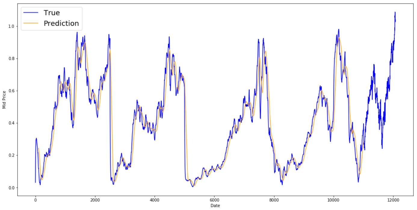
Take a look at the averaged results below. They follow the stock's actual behavior quite closely. Next, you will examine a more accurate one-step prediction method.
plt.figure(figsize = (18,9))
plt.plot(range(df.shape[0]),all_mid_data,color='b',label='True')
plt.plot(range(window_size,N),std_avg_predictions,color='orange',label='Prediction')
#plt.xticks(range(0,df.shape[0],50),df['Date'].loc[::50],rotation=45)
plt.xlabel('Date')
plt.ylabel('Mid Price')
plt.legend(fontsize=18)
plt.show()
So what do the above graphs (and the MSE) say?
It seems that it is not too bad of a model for very short predictions (one day ahead). This behavior is sensible since stock prices don't change from 0 to 100 overnight. Next, you will look at a fancier averaging technique, the exponential moving average.
Exponential moving average
You might have seen some articles on the internet using very complex models and predicting almost the exact behavior of the stock market. But beware! These are just optical illusions and not due to learning something useful. You will see below how you can replicate that behavior with a simple averaging method.
In the exponential moving average method, you calculate $x_{t+1}$ as,
- $x\_{t+1} = EMA\_{t} = \gamma \times EMA_{t-1} + (1-\gamma) x_t$ where $EMA_0 = 0$ and $EMA$ is the exponential moving average value you maintain over time.
The above equation basically calculates the exponential moving average from $t+1$ time step and uses that as the one step ahead prediction. $\gamma$ decides what the contribution of the most recent prediction is to the EMA. For example, a $\gamma=0.1$ gets only 10% of the current value into the EMA. Because you take only a very small fraction of the most recent, it allows to preserve much older values you saw very early in the average. See how good this looks when used to predict one-step ahead below.
window_size = 100
N = train_data.size

run_avg_predictions = []
run_avg_x = []

mse_errors = []

running_mean = 0.0
run_avg_predictions.append(running_mean)

decay = 0.5

for pred_idx in range(1,N):

    running_mean = running_mean*decay + (1.0-decay)*train_data[pred_idx-1]
    run_avg_predictions.append(running_mean)
    mse_errors.append((run_avg_predictions[-1]-train_data[pred_idx])**2)
    run_avg_x.append(date)

print('MSE error for EMA averaging: %.5f'%(0.5*np.mean(mse_errors)))
MSE error for EMA averaging: 0.00003
plt.figure(figsize = (18,9))
plt.plot(range(df.shape[0]),all_mid_data,color='b',label='True')
plt.plot(range(0,N),run_avg_predictions,color='orange', label='Prediction')
#plt.xticks(range(0,df.shape[0],50),df['Date'].loc[::50],rotation=45)
plt.xlabel('Date')
plt.ylabel('Mid Price')
plt.legend(fontsize=18)
plt.show()
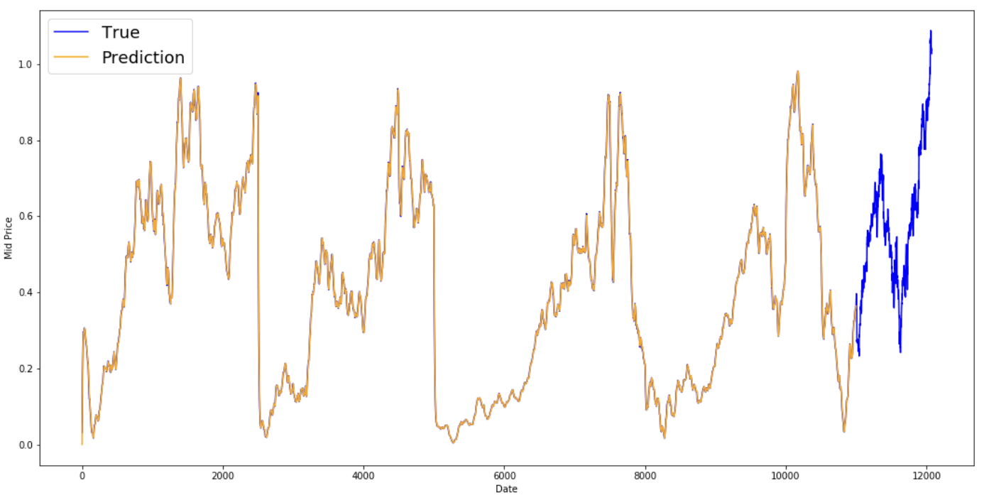
If the exponential moving average is this good, why do you need better models?
You see that it fits a perfect line that follows the True distribution (and justified by the very low MSE). Practically speaking, you can't do much with just the stock market value of the next day. Personally, what I'd like is not the exact stock market price for the next day, but would the stock market prices go up or down in the next 30 days? Try to do this, and you will expose the incapability of the EMA method.
You will now try to make predictions in windows (say you predict the next 2 days window, instead of just the next day). Then, you will realize how wrong EMA can go. Here is an example:
Predict more than one step into the future
To make things concrete, let's assume values, say $x_t=0.4$, $EMA=0.5$ and $\gamma = 0.5$
- Say you get the output with the following equation
- Xt+1 = EMAt = γ × EMAt-1 + (1 - γ)Xt
- So you have xt+1 = 0.5 × 0.5 + (1-0.5) × 0.4 = 0.45
- So Xt+1 = EMAt = 0.45
- So the next prediction Xt+2 becomes,
- Xt+2 = γ × EMAt + (1-γ)Xt+1
- Which is Xt+2 = γ × EMA_t + (1-γ) EMAt = EMAt
- Or in this example, Xt+2 = Xt+1 = 0.45
So, no matter how many steps you predict in the future, you'll keep getting the same answer for all the future prediction steps.
One solution you have that will output useful information is to look at momentum-based algorithms. They make predictions based on whether the past recent values were going up or going down (not the exact values). For example, they will say the next-day price will likely be lower if the prices have been dropping for the past few days, which sounds reasonable. However, you will use a more complex model: an LSTM model.
These models have taken the realm of time series prediction by storm because they are so good at modeling time series data. You will see if there actually are patterns hidden in the data that you can exploit.
Introduction to LSTMs: Making Stock Movement Predictions Far into the Future
Long-short-term memory models are extremely powerful time-series models. They can predict an arbitrary number of steps into the future. An LSTM module (or cell) has 5 essential components, which allow it to model both long-term and short-term data.
- Cell state (ct) - This represents the internal memory of the cell, which stores both short-term memory and long-term memories.
- Hidden state (ht) - This is output state information calculated w.r.t. current input, previous hidden state, and current cell input, which you eventually use to predict the future stock market prices. Additionally, the hidden state can decide to only retrieve short- or long-term memories or both types of memory stored in the cell state to make the next prediction.
- Input gate (it) - Decides how much information from current input flows to the cell state.
- Forget gate (ft) - Decides how much information from the current input and the previous cell state flows into the current cell state.
- Output gate (ot) - Decides how much information from the current cell state flows into the hidden state so that if needed LSTM can only pick the long-term memories or short-term memories and long-term memories.
A cell is pictured below:
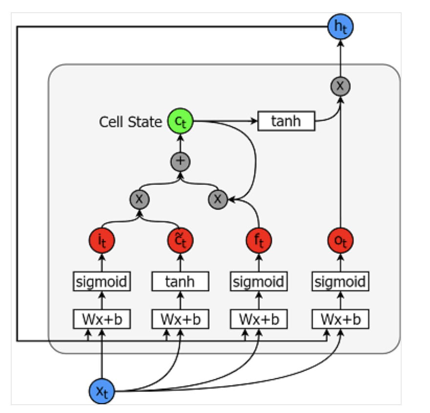
The equations for calculating each of these entities are as follows.
- it = σ(WixXt + Wihht-1 + bi)
- $\tilde{c}\_t = \sigma(W\_{cx}x\_t + W\_{ch}h_{t-1} + b_c)$
- $f\_t = \sigma(W\_{fx}x\_t + W\_{fh}h_{t-1}+b_f)$
- $c_t = f\_t c\_{t-1} + i_t \tilde{c}_t$
- $o\_t = \sigma(W\_{ox}x\_t + W\_{oh}h_{t-1}+b_o)$
- $h_t = o_t tanh(c_t)$
You can refer to this article for a better (more technical) understanding of LSTMs.
TensorFlow provides a nice API (called RNN API) for implementing time series models. You will be using that for your implementations.
Data generator
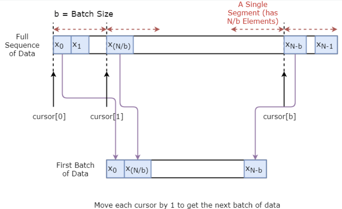
You are first going to implement a data generator to train your model. This data generator will have a method called .unroll_batches(...) which will output a set of num_unrollings batches of input data obtained sequentially, where a batch of data is of size [batch_size, 1]. Then, each batch of input data will have a corresponding output batch of data.
For example if num_unrollings=3 and batch_size=4 a set of unrolled batches it might look like,
- input data: $[x_0,x_10,x_20,x_30], [x_1,x_11,x_21,x_31], [x_2,x_12,x_22,x_32]$
- output data: $[x_1,x_11,x_21,x_31], [x_2,x_12,x_22,x_32], [x_3,x_13,x_23,x_33]$
Data augmentation
Also, to make your model robust, you will not make the output for $x\_t$ always $x\_{t+1}$. Rather you will randomly sample an output from the set $x\_{t+1},x\_{t+2},\ldots,x_{t+N}$ where $N$ is a small window size.
Here, you are making the following assumption:
- $x\_{t+1},x\_{t+2},\ldots,x_{t+N}$ will not be very far from each other
I personally think this is a reasonable assumption for stock movement predictions.
Below, you illustrate how a batch of data is created visually.
class DataGeneratorSeq(object):

    def __init__(self,prices,batch_size,num_unroll):
        self._prices = prices
        self._prices_length = len(self._prices) - num_unroll
        self._batch_size = batch_size
        self._num_unroll = num_unroll
        self._segments = self._prices_length //self._batch_size
        self._cursor = [offset * self._segments for offset in range(self._batch_size)]

    def next_batch(self):

        batch_data = np.zeros((self._batch_size),dtype=np.float32)
        batch_labels = np.zeros((self._batch_size),dtype=np.float32)

        for b in range(self._batch_size):
            if self._cursor[b]+1>=self._prices_length:
                #self._cursor[b] = b * self._segments
                self._cursor[b] = np.random.randint(0,(b+1)*self._segments)

            batch_data[b] = self._prices[self._cursor[b]]
            batch_labels[b]= self._prices[self._cursor[b]+np.random.randint(0,5)]

            self._cursor[b] = (self._cursor[b]+1)%self._prices_length

        return batch_data,batch_labels

    def unroll_batches(self):

        unroll_data,unroll_labels = [],[]
        init_data, init_label = None,None
        for ui in range(self._num_unroll):

            data, labels = self.next_batch()

            unroll_data.append(data)
            unroll_labels.append(labels)

        return unroll_data, unroll_labels

    def reset_indices(self):
        for b in range(self._batch_size):
            self._cursor[b] = np.random.randint(0,min((b+1)*self._segments,self._prices_length-1))


dg = DataGeneratorSeq(train_data,5,5)
u_data, u_labels = dg.unroll_batches()

for ui,(dat,lbl) in enumerate(zip(u_data,u_labels)):
    print('\n\nUnrolled index %d'%ui)
    dat_ind = dat
    lbl_ind = lbl
    print('\tInputs: ',dat )
    print('\n\tOutput:',lbl)
Unrolled index 0
    Inputs:  [0.03143791 0.6904868  0.82829314 0.32585657 0.11600105]

    Output: [0.08698314 0.68685144 0.8329321  0.33355275 0.11785509]


Unrolled index 1
    Inputs:  [0.06067836 0.6890754  0.8325337  0.32857886 0.11785509]

    Output: [0.15261841 0.68685144 0.8325337  0.33421066 0.12106793]


Unrolled index 2
    Inputs:  [0.08698314 0.68685144 0.8329321  0.33078218 0.11946969]

    Output: [0.11098009 0.6848606  0.83387965 0.33421066 0.12106793]


Unrolled index 3
    Inputs:  [0.11098009 0.6858036  0.83294916 0.33219692 0.12106793]

    Output: [0.132895   0.6836884  0.83294916 0.33219692 0.12288672]


Unrolled index 4
    Inputs:  [0.132895   0.6848606  0.833369   0.33355275 0.12158521]

    Output: [0.15261841 0.6836884  0.83383167 0.33355275 0.12230608]
Defining hyperparameters
In this section, you'll define several hyperparameters. D is the dimensionality of the input. It's straightforward, as you take the previous stock price as the input and predict the next one, which should be 1.
Then you have num_unrollings, this is a hyperparameter related to the backpropagation through time (BPTT) that is used to optimize the LSTM model. This denotes how many continuous time steps you consider for a single optimization step. You can think of this as, instead of optimizing the model by looking at a single time step, you optimize the network by looking at num_unrollings time steps. The larger the better.
Then you have the batch_size. Batch size is how many data samples you consider in a single time step.
Next you define num_nodes which represents the number of hidden neurons in each cell. You can see that there are three layers of LSTMs in this example.
D = 1 # Dimensionality of the data. Since your data is 1-D this would be 1
num_unrollings = 50 # Number of time steps you look into the future.
batch_size = 500 # Number of samples in a batch
num_nodes = [200,200,150] # Number of hidden nodes in each layer of the deep LSTM stack we're using
n_layers = len(num_nodes) # number of layers
dropout = 0.2 # dropout amount

tf.reset_default_graph() # This is important in case you run this multiple times
Defining inputs and outputs
Next, you define placeholders for training inputs and labels. This is very straightforward as you have a list of input placeholders, each containing a single batch of data. And the list has num_unrollings placeholders, that will be used at once for a single optimization step.
# Input data.
train_inputs, train_outputs = [],[]

# You unroll the input over time defining placeholders for each time step
for ui in range(num_unrollings):
    train_inputs.append(tf.placeholder(tf.float32, shape=[batch_size,D],name='train_inputs_%d'%ui))
    train_outputs.append(tf.placeholder(tf.float32, shape=[batch_size,1], name = 'train_outputs_%d'%ui))
Defining parameters of the LSTM and regression layer
You will have a three layers of LSTMs and a linear regression layer, denoted by w and b, that takes the output of the last Long Short-Term Memory cell and output the prediction for the next time step. You can use the MultiRNNCell in TensorFlow to encapsulate the three LSTMCell objects you created. Additionally, you can have the dropout implemented LSTM cells, as they improve performance and reduce overfitting.
lstm_cells = [
    tf.contrib.rnn.LSTMCell(num_units=num_nodes[li],
                            state_is_tuple=True,
                            initializer= tf.contrib.layers.xavier_initializer()
                           )
 for li in range(n_layers)]

drop_lstm_cells = [tf.contrib.rnn.DropoutWrapper(
    lstm, input_keep_prob=1.0,output_keep_prob=1.0-dropout, state_keep_prob=1.0-dropout
) for lstm in lstm_cells]
drop_multi_cell = tf.contrib.rnn.MultiRNNCell(drop_lstm_cells)
multi_cell = tf.contrib.rnn.MultiRNNCell(lstm_cells)

w = tf.get_variable('w',shape=[num_nodes[-1], 1], initializer=tf.contrib.layers.xavier_initializer())
b = tf.get_variable('b',initializer=tf.random_uniform([1],-0.1,0.1))
Calculating LSTM output and feeding it to the regression layer to get the final prediction
In this section, you first create TensorFlow variables (c and h) that will hold the cell state and the hidden state of the Long Short-Term Memory cell. Then you transform the list of train_inputs to have a shape of [num_unrollings, batch_size, D], this is needed for calculating the outputs with the tf.nn.dynamic_rnn function. You then calculate the LSTM outputs with the tf.nn.dynamic_rnn function and split the output back to a list of num_unrolling tensors. the loss between the predictions and true stock prices.
# Create cell state and hidden state variables to maintain the state of the LSTM
c, h = [],[]
initial_state = []
for li in range(n_layers):
  c.append(tf.Variable(tf.zeros([batch_size, num_nodes[li]]), trainable=False))
  h.append(tf.Variable(tf.zeros([batch_size, num_nodes[li]]), trainable=False))
  initial_state.append(tf.contrib.rnn.LSTMStateTuple(c[li], h[li]))

# Do several tensor transofmations, because the function dynamic_rnn requires the output to be of
# a specific format. Read more at: https://www.tensorflow.org/api_docs/python/tf/nn/dynamic_rnn
all_inputs = tf.concat([tf.expand_dims(t,0) for t in train_inputs],axis=0)

# all_outputs is [seq_length, batch_size, num_nodes]
all_lstm_outputs, state = tf.nn.dynamic_rnn(
    drop_multi_cell, all_inputs, initial_state=tuple(initial_state),
    time_major = True, dtype=tf.float32)

all_lstm_outputs = tf.reshape(all_lstm_outputs, [batch_size*num_unrollings,num_nodes[-1]])

all_outputs = tf.nn.xw_plus_b(all_lstm_outputs,w,b)

split_outputs = tf.split(all_outputs,num_unrollings,axis=0)
Loss calculation and optimizer
Now, you'll calculate the loss. However, you should note that there is a unique characteristic when calculating the loss. For each batch of predictions and true outputs, you calculate the Mean Squared Error. And you sum (not average) all these mean squared losses together. Finally, you define the optimizer you're going to use to optimize the neural network. In this case, you can use Adam, which is a very recent and well-performing optimizer.
# When calculating the loss you need to be careful about the exact form, because you calculate
# loss of all the unrolled steps at the same time
# Therefore, take the mean error or each batch and get the sum of that over all the unrolled steps

print('Defining training Loss')
loss = 0.0
with tf.control_dependencies([tf.assign(c[li], state[li][0]) for li in range(n_layers)]+
                             [tf.assign(h[li], state[li][1]) for li in range(n_layers)]):
  for ui in range(num_unrollings):
    loss += tf.reduce_mean(0.5*(split_outputs[ui]-train_outputs[ui])**2)

print('Learning rate decay operations')
global_step = tf.Variable(0, trainable=False)
inc_gstep = tf.assign(global_step,global_step + 1)
tf_learning_rate = tf.placeholder(shape=None,dtype=tf.float32)
tf_min_learning_rate = tf.placeholder(shape=None,dtype=tf.float32)

learning_rate = tf.maximum(
    tf.train.exponential_decay(tf_learning_rate, global_step, decay_steps=1, decay_rate=0.5, staircase=True),
    tf_min_learning_rate)

# Optimizer.
print('TF Optimization operations')
optimizer = tf.train.AdamOptimizer(learning_rate)
gradients, v = zip(*optimizer.compute_gradients(loss))
gradients, _ = tf.clip_by_global_norm(gradients, 5.0)
optimizer = optimizer.apply_gradients(
    zip(gradients, v))

print('\tAll done')
Defining training Loss
Learning rate decay operations
TF Optimization operations
    All done
Prediction related calculations
Here you define the prediction related TensorFlow operations. First, define a placeholder for feeding in the input (sample_inputs), then similar to the training stage, you define state variables for prediction (sample_c and sample_h). Finally you calculate the prediction with the tf.nn.dynamic_rnn function and then sending the output through the regression layer (w and b). You also should define the reset_sample_state operation, which resets the cell state and the hidden state. You should execute this operation at the start, every time you make a sequence of predictions.
print('Defining prediction related TF functions')

sample_inputs = tf.placeholder(tf.float32, shape=[1,D])

# Maintaining LSTM state for prediction stage
sample_c, sample_h, initial_sample_state = [],[],[]
for li in range(n_layers):
  sample_c.append(tf.Variable(tf.zeros([1, num_nodes[li]]), trainable=False))
  sample_h.append(tf.Variable(tf.zeros([1, num_nodes[li]]), trainable=False))
  initial_sample_state.append(tf.contrib.rnn.LSTMStateTuple(sample_c[li],sample_h[li]))

reset_sample_states = tf.group(*[tf.assign(sample_c[li],tf.zeros([1, num_nodes[li]])) for li in range(n_layers)],
                               *[tf.assign(sample_h[li],tf.zeros([1, num_nodes[li]])) for li in range(n_layers)])

sample_outputs, sample_state = tf.nn.dynamic_rnn(multi_cell, tf.expand_dims(sample_inputs,0),
                                   initial_state=tuple(initial_sample_state),
                                   time_major = True,
                                   dtype=tf.float32)

with tf.control_dependencies([tf.assign(sample_c[li],sample_state[li][0]) for li in range(n_layers)]+
                              [tf.assign(sample_h[li],sample_state[li][1]) for li in range(n_layers)]):
  sample_prediction = tf.nn.xw_plus_b(tf.reshape(sample_outputs,[1,-1]), w, b)

print('\tAll done')
Defining prediction related TF functions
    All done
Running the LSTM
Here you will train and predict stock price movements for several epochs and see whether the predictions get better or worse over time. You follow the following procedure.
- Define a test set of starting points (
test_points_seq) on the time series to evaluate the model on - For each epoch
- For full sequence length of training data
- Unroll a set of
num_unrollingsbatches - Train the neural network with the unrolled batches
- Unroll a set of
- Calculate the average training loss
- For each starting point in the test set
- Update the LSTM state by iterating through the previous
num_unrollingsdata points found before the test point - Make predictions for
n_predict_oncesteps continuously, using the previous prediction as the current input - Calculate the MSE loss between the
n_predict_oncepoints predicted and the true stock prices at those time stamps
- Update the LSTM state by iterating through the previous
- For full sequence length of training data
epochs = 30
valid_summary = 1 # Interval you make test predictions

n_predict_once = 50 # Number of steps you continously predict for

train_seq_length = train_data.size # Full length of the training data

train_mse_ot = [] # Accumulate Train losses
test_mse_ot = [] # Accumulate Test loss
predictions_over_time = [] # Accumulate predictions

session = tf.InteractiveSession()

tf.global_variables_initializer().run()

# Used for decaying learning rate
loss_nondecrease_count = 0
loss_nondecrease_threshold = 2 # If the test error hasn't increased in this many steps, decrease learning rate

print('Initialized')
average_loss = 0

# Define data generator
data_gen = DataGeneratorSeq(train_data,batch_size,num_unrollings)

x_axis_seq = []

# Points you start your test predictions from
test_points_seq = np.arange(11000,12000,50).tolist()

for ep in range(epochs):

    # ========================= Training =====================================
    for step in range(train_seq_length//batch_size):

        u_data, u_labels = data_gen.unroll_batches()

        feed_dict = {}
        for ui,(dat,lbl) in enumerate(zip(u_data,u_labels)):
            feed_dict[train_inputs[ui]] = dat.reshape(-1,1)
            feed_dict[train_outputs[ui]] = lbl.reshape(-1,1)

        feed_dict.update({tf_learning_rate: 0.0001, tf_min_learning_rate:0.000001})

        _, l = session.run([optimizer, loss], feed_dict=feed_dict)

        average_loss += l

    # ============================ Validation ==============================
    if (ep+1) % valid_summary == 0:

      average_loss = average_loss/(valid_summary*(train_seq_length//batch_size))

      # The average loss
      if (ep+1)%valid_summary==0:
        print('Average loss at step %d: %f' % (ep+1, average_loss))

      train_mse_ot.append(average_loss)

      average_loss = 0 # reset loss

      predictions_seq = []

      mse_test_loss_seq = []

      # ===================== Updating State and Making Predicitons ========================
      for w_i in test_points_seq:
        mse_test_loss = 0.0
        our_predictions = []

        if (ep+1)-valid_summary==0:
          # Only calculate x_axis values in the first validation epoch
          x_axis=[]

        # Feed in the recent past behavior of stock prices
        # to make predictions from that point onwards
        for tr_i in range(w_i-num_unrollings+1,w_i-1):
          current_price = all_mid_data[tr_i]
          feed_dict[sample_inputs] = np.array(current_price).reshape(1,1)
          _ = session.run(sample_prediction,feed_dict=feed_dict)

        feed_dict = {}

        current_price = all_mid_data[w_i-1]

        feed_dict[sample_inputs] = np.array(current_price).reshape(1,1)

        # Make predictions for this many steps
        # Each prediction uses previous prediciton as it's current input
        for pred_i in range(n_predict_once):

          pred = session.run(sample_prediction,feed_dict=feed_dict)

          our_predictions.append(np.asscalar(pred))

          feed_dict[sample_inputs] = np.asarray(pred).reshape(-1,1)

          if (ep+1)-valid_summary==0:
            # Only calculate x_axis values in the first validation epoch
            x_axis.append(w_i+pred_i)

          mse_test_loss += 0.5*(pred-all_mid_data[w_i+pred_i])**2

        session.run(reset_sample_states)

        predictions_seq.append(np.array(our_predictions))

        mse_test_loss /= n_predict_once
        mse_test_loss_seq.append(mse_test_loss)

        if (ep+1)-valid_summary==0:
          x_axis_seq.append(x_axis)

      current_test_mse = np.mean(mse_test_loss_seq)

      # Learning rate decay logic
      if len(test_mse_ot)>0 and current_test_mse > min(test_mse_ot):
          loss_nondecrease_count += 1
      else:
          loss_nondecrease_count = 0

      if loss_nondecrease_count > loss_nondecrease_threshold :
            session.run(inc_gstep)
            loss_nondecrease_count = 0
            print('\tDecreasing learning rate by 0.5')

      test_mse_ot.append(current_test_mse)
      print('\tTest MSE: %.5f'%np.mean(mse_test_loss_seq))
      predictions_over_time.append(predictions_seq)
      print('\tFinished Predictions')
Initialized
Average loss at step 1: 1.703350
    Test MSE: 0.00318
    Finished Predictions
  ...
  ...
  ...
Average loss at step 30: 0.033753
    Test MSE: 0.00243
    Finished Predictions
Visualizing the Predictions
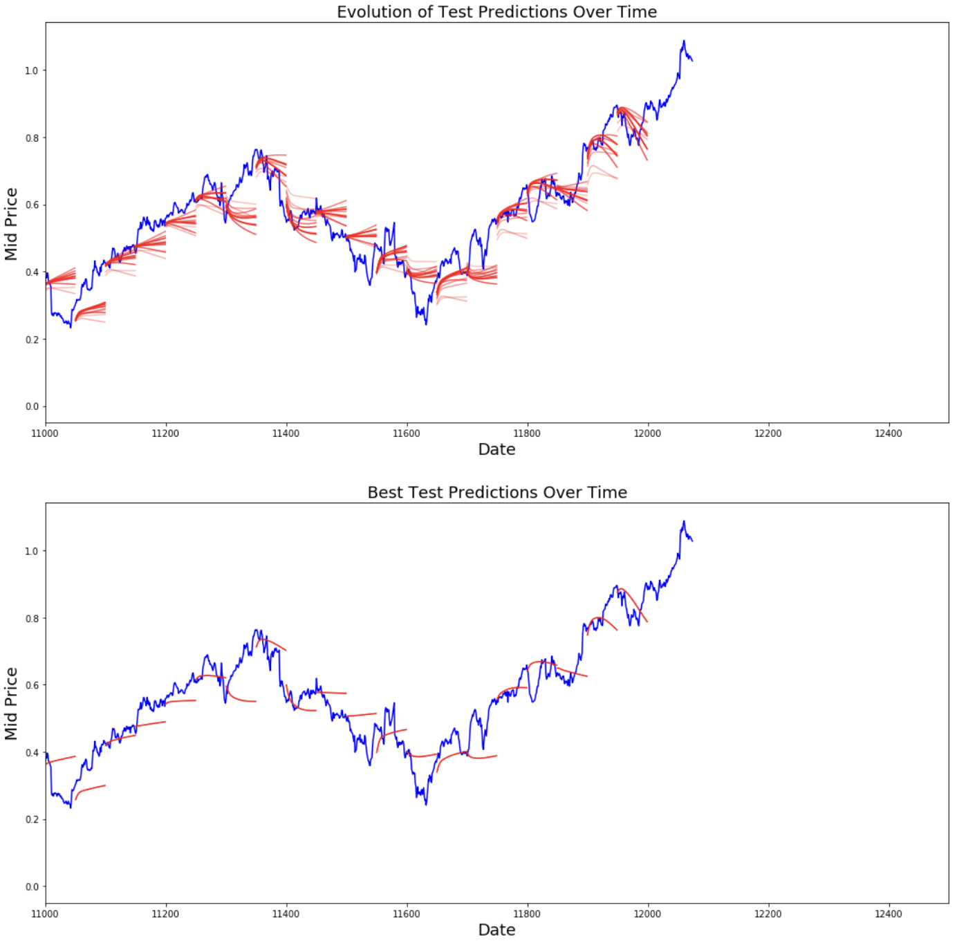
You can see how the MSE loss is going down with the amount of training. This is a good sign that the model is learning something useful. To quantify your findings, you can compare the network's MSE loss to the MSE loss you obtained when doing the standard averaging (0.004). You can see that the LSTM is doing better than the standard averaging. And you know that standard averaging (though not perfect) followed the true stock prices movements reasonably.
best_prediction_epoch = 28 # replace this with the epoch that you got the best results when running the plotting code

plt.figure(figsize = (18,18))
plt.subplot(2,1,1)
plt.plot(range(df.shape[0]),all_mid_data,color='b')

# Plotting how the predictions change over time
# Plot older predictions with low alpha and newer predictions with high alpha
start_alpha = 0.25
alpha  = np.arange(start_alpha,1.1,(1.0-start_alpha)/len(predictions_over_time[::3]))
for p_i,p in enumerate(predictions_over_time[::3]):
    for xval,yval in zip(x_axis_seq,p):
        plt.plot(xval,yval,color='r',alpha=alpha[p_i])

plt.title('Evolution of Test Predictions Over Time',fontsize=18)
plt.xlabel('Date',fontsize=18)
plt.ylabel('Mid Price',fontsize=18)
plt.xlim(11000,12500)

plt.subplot(2,1,2)

# Predicting the best test prediction you got
plt.plot(range(df.shape[0]),all_mid_data,color='b')
for xval,yval in zip(x_axis_seq,predictions_over_time[best_prediction_epoch]):
    plt.plot(xval,yval,color='r')

plt.title('Best Test Predictions Over Time',fontsize=18)
plt.xlabel('Date',fontsize=18)
plt.ylabel('Mid Price',fontsize=18)
plt.xlim(11000,12500)
plt.show()
Though not perfect, LSTMs seem to be able to predict stock price behavior correctly most of the time. Note that you are making predictions roughly in the range of 0 and 1.0 (that is, not the true stock prices). This is okay because you're predicting the stock price movement, not the prices themselves.
Final Remarks
I'm hoping that you found this tutorial useful. I should mention that this was a rewarding experience for me. In this tutorial, I learned how difficult it can be to devise a model that is able to predict stock price movements correctly. You started with a motivation for why you need to model stock prices. This was followed by an explanation and code for downloading data. Then, you looked at two averaging techniques that allow you to make predictions one step into the future. You next saw that these methods are futile when you need to predict more than one step into the future. Thereafter, you discussed how you can use LSTMs to make predictions for many steps into the future. Finally, you visualized the results and saw that your model (though not perfect) is quite good at correctly predicting stock price movements.
If you would like to learn more about deep learning, be sure to take a look at our Deep Learning in Python course. It covers the basics, as well as how to build a neural network on your own in Keras. This is a different package than TensorFlow, which will be used in this tutorial, but the idea is the same.
Here, I'm stating several takeaways from this tutorial.
-
Stock price/movement prediction is an extremely difficult task. Personally, I don't think any of the stock prediction models out there shouldn't be taken for granted and blindly rely on them. However, models might be able to predict stock price movement correctly most of the time, but not always.
-
Do not be fooled by articles out there that shows predictions curves that perfectly overlaps the true stock prices. This can be replicated with a simple averaging technique and in practice it's useless. A more sensible thing to do is predicting the stock price movements.
-
The model's hyperparameters are extremely sensitive to the results you obtain. So, a very good thing to do would be to run some hyperparameter optimization techniques (for example, Grid search / Random search) on the hyperparameters. Below, I listed some of the most critical hyperparameters:
- The learning rate of the optimizer
- The number of layers and the number of hidden units in each layer
- The optimizer. I found Adam to perform the best
- Type of the model. You can try GRU/ Standard LSTM/ LSTM with Peepholes and evaluation performance difference
-
In this tutorial you did something faulty (due to the small size of data)! That is you used the test loss to decay the learning rate. This indirectly leaks information about test set into the training procedure. A better way of handling this is to have a separate validation set (apart from the test set) and decay learning rate with respect to performance of the validation set.
If you'd like to get in touch with me, you can drop me an e-mail at thushv@gmail.com or connect with me on LinkedIn.
References
I referred to this repository to get an understanding about how to use LSTMs for stock predictions. But details can be vastly different from the implementation found in the reference.
Build Machine Learning Skills
FAQs
Can LSTM models guarantee accurate stock market predictions?
No, LSTM models cannot guarantee accurate predictions because the stock market is highly volatile and influenced by factors beyond historical data. LSTMs can help identify trends and patterns but should not be solely relied upon for financial decisions.
How does normalization improve LSTM predictions for stock data?
Normalization ensures that data values fall within a similar range, reducing the influence of outliers and improving model performance. It helps the LSTM focus on patterns rather than absolute values, which is crucial for training.
Why use exponential moving averages (EMA) before introducing LSTMs?
Exponential moving averages smooth out fluctuations in stock data, providing a clearer view of trends. This step serves as a baseline for comparison and highlights the limitations of simpler methods versus LSTMs.
What are some limitations of the approach outlined in this tutorial?
This tutorial assumes access to sufficient and clean historical data. The model's performance is also limited by the chosen hyperparameters, data preprocessing steps, and the unpredictable nature of real-world stock movements.
Can the LSTM model predict stock movements for individual companies equally well?
Not necessarily. The model's accuracy depends on the characteristics of the stock data, such as volatility and liquidity. Testing and fine-tuning are required for each specific stock to achieve optimal results.

