Ensemble Modeling Tutorial: Explore Ensemble Learning Techniques

Machine learning models are not like traditional software solutions.  These models need constant updates as new data becomes available for accurate and reliable predictions. In complex and sensitive scenarios, relying on a single model may  not be sufficient to generate an optimal result,  and this is where ensemble modeling can help. 

This conceptual tutorial covers what ensemble modeling in machine learning is and how it can improve your overall model performance. Then, we’ll provide an overview of various ensemble methods before diving into the illustration of a real-world scenario using a step-by-step implementation with Python.

Our Ensemble Learning in R with SuperLearner tutorial explains how to boost your machine learning results and based on ensemble learning approach using the SuperLearner package in R.

Ensemble Models in Machine Learning

Let’s imagine a music manager participating in an international competition.  They have access to a wide variety of musicians with different expertise: 

• Classical musicians with the ability to compose traditional pieces.
• Electronic musicians who are experts in using electronic instruments.
• Jazz musicians with a great sense of improvisation.
• Soloist musicians who can perform complex solos and highlight their technical abilities.

Given the broad spectrum of musical expertise and background, the manager can combine all of them to create a unique and memorable performance.

Think of ensemble models as an orchestra of musicians, where each person specializes in a specific instrument like piano, trumpet, drum, and more. The combination of those skills creates a harmonious melody. 

Ensemble learning uses the same logic: 

It combines multiple algorithms to obtain better predictive performance than the one from a single model. There is no predefined number of models to consider, and some business goals may require more models than others.

Model Error and Reducing this Error with Ensembles

The error emerging from any machine model can be broken down into three components mathematically:

Bias + Variance + Irreducible error

Why is this important in the current context? To understand what goes on behind an ensemble model, you need first to know what causes an error in the model. 

Let’s look at these errors: 

Bias error 

This is useful to quantify how much, on an average, the predicted values are different from the actual value. A high bias error means we have an underperforming model that keeps missing essential trends.

Variance

On the other side, Variance quantifies how the predictions made on the same observation differ. A high variance model will over-fit on your training population and perform poorly on any observation beyond training. The following diagram will give you more clarity (assume that the red spot is the real value, and the blue dots are predictions): 

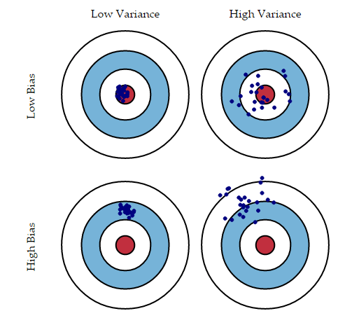
Typically, as you increase the complexity of your model, you will see a reduction in error due to lower bias in the model. However, this only happens until a particular point. As you continue to make your model more complex, you end up over-fitting your model, and hence your model will start suffering from the high variance.

Now that you are familiar with the basics of ensemble learning let's look at different ensemble learning techniques:

Types of Ensemble Methods

There are different types of ensemble methods, and each one brings a set of advantages and disadvantages. This section covers those aspects to help you make the right choice for your use cases. 

Before diving into each method, let’s understand what meta and base learners are for a better understanding of the next concepts. 

• Base learners are the first level of an ensemble learning architecture, and each one of them is trained to make individual predictions. 
• Meta learners, on the other hand, are in the second level, and they are trained on the output of the base learners. 

Bagging

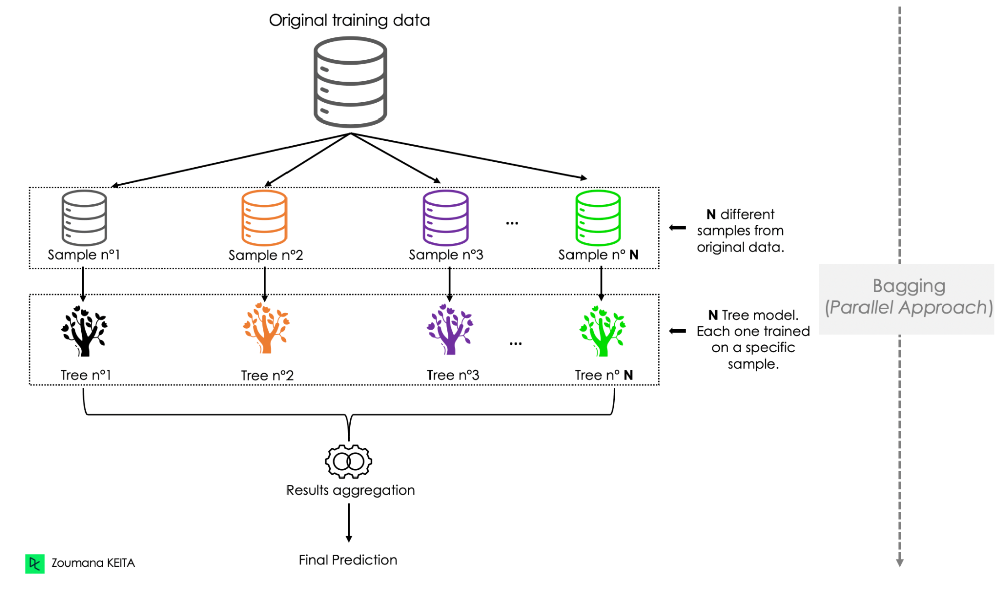
Bagging is also known as bootstrap aggregation.  This technique is similar to random forest, but it uses all the predictors, whereas random forest uses only a subset of predictors in each tree.  

In bagging, a random sample of data from the training set is selected with replacement, which enables the duplication of sample instances in a set. Below are the main steps involved in bagging: 

• Generation of multiple bootstrap resamples.
• Running an algorithm on each resample to make predictions.
• Combining the predictions by taking the average of the predictions or taking the majority vote (for classification).

Bagging presents several key advantages and disadvantages when used for classification or regression tasks.

Advantages

• The modeling process is straightforward and does not require any deep mathematical concepts, and can handle missing values.
• The scikit-learn package makes it easy to implement the underlying logic. It contains all the modules to combine the predictions of each model, also known as base learners. 
• It has a significant effect on reducing variance on high-variance classifiers. This is helpful when dealing with high-dimensional data, preventing the model from accurately generalizing on new data. 
• Bagging provides an unbiased estimate of the out-of-bag error, which corresponds to the average error/loss that all these classifiers yield.

Disadvantages

• Bagging is computationally expensive due to the use of several models.
• The averaging involved across predictions makes it difficult to interpret the final result.

Boosting

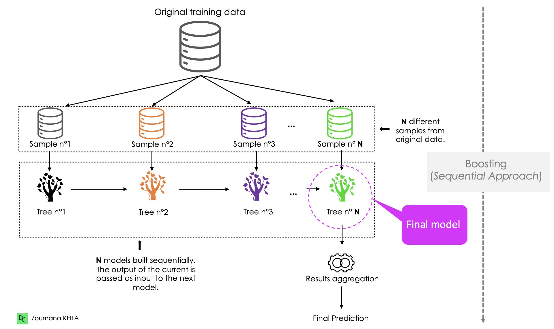
Boosting adopts a sequential approach, where the prediction of the current model is transferred to the next one. Each model iteratively focuses attention on the observations that are misclassified by its predecessors. We’ve outlined the general process below: 

Advantages

• Similarly to bagging, boosting is easy to understand and implement. Furthermore, it does not require any preprocessing and can handle missing values in the data.
• It efficiently reduces bias. 
• Boosting algorithms prioritize features that increase overall accuracy during the training. This process reduces the dimensionality of the data, hence reducing the computation time. 

Disadvantages

• The sequential approach of boosting makes the next models correct the mistakes of its predecessor. This makes the overall model vulnerable to outliers.
• Boosting is not scalable for the same reason as the sequential aspect.

Stacking

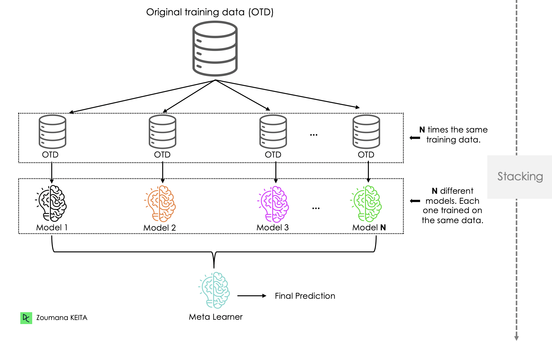
Stacking is pretty similar to boosting. The predictions from the base learners are stacked together and are used as the input to train the meta learner to produce more robust predictions. The meta learner is then used to make final predictions. Bagging and boosting typically use homogeneous base learners, whereas stacking tends to include heterogeneous ones. 

Advantages

• It leverages the strengths of multiple high-performing models for both classification and regression tasks.
• Similar to other ensemble models, stacking helps build a more accurate model than individual models used alone.

Disadvantages

• Using complex basic models can increase the risk of overfitting.
• Different levels of a model’s training can make the stacking architecture complex to implement.

Blending 

Blending is similar to Stacking. In blending, the structure of the data is made of training, hold-out, and test data. The meta learners are trained on the training data. Then their predictions are combined with the hold-out data to build the final meta model, which uses the test data to make the final predictions.

Advantages

• Like stacking and many other ensemble methods, blending can boost the final model’s performance in many cases. 
• This use of this technique has been successful in winning many competitions. 

Disadvantages

• Dividing the original data according to the blending architecture can limit the use of data for training base models, hence resulting in poor performance.
• Like other ensemble models, the final model interpretability is reduced due to increased complexity, hence making it difficult to draw any crucial business insights.

Voting

In voting, multiple models are trained independently, and their predictions are combined to make a final prediction using either hard voting, soft voting, or weighted voting:

• In hard voting, the final prediction is the most common prediction from all the models.  
• For soft voting, each model generates a probability distribution instead of a binary prediction. Then, the class with the highest probability is the one predicted. 
• Finally, in weighted voting, there is an assumption that some models have more skill than other,s and those models are assigned with more contribution when making predictions.

Advantages

• Voting architecture is simple to implement compared to stacking, and blending. Also, it does not require complex fine-tuning. 
• Using multiple base learners in the voting makes it less susceptible to the influence of individual models, which contributes to making more stable and reliable predictions.

Disadvantages

• It can be difficult to deal with models’ prediction conflict, which makes it hard to make the final decision in a meaningful way.
• Adding more models to the ensemble voting model does not necessarily improve the final performance.

Cascading 

Cascading uses a stacking approach but with only one model in each layer. The first model is trained on the whole training data, and the next model is trained on the output of the model before. The goal of using the strategy is to learn complex patterns from the data, hence allow the model to make better predictions.   

Advantages

• The next model is specialized in the output of the previous model, which reduces noise in the data.
• More robust to overfitting and can perform well on real-world data.

Disadvantages

• Implementing the cascading can be complex since it involves training each of the modes in the sequence.  
• Getting the optimal cascading architecture can require a lot of experimentation and fine-tuning.

Overview of Ensemble Algorithms

The previous sections covered the different types of ensemble models. Now, let’s have a brief overview of some popular models. 

Random Forest

Random Forest is a commonly used model that can solve both classification and regression problems. A random forest is made up of many decision trees that are trained using bagging. Its outcome is determined by taking the average of the prediction of individual trees. 

The node size, the number of trees, and number of features sampled are the three main hyperparameters that need to be set before training the random forest. 

What about randomness in a random forest?

Feature bagging, also known as feature randomness, creates a random sample of features to ensure low correlation among decision trees. This approach sets apart random forests from decision trees which consider all the possible feature splits, whereas random forests consider only a subset of those features. Read in our random forest classification tutorial. 

XGBoost

Extreme Gradient Boosting, or XGBoost for short, is used for both classification and regression. XGBoost is designed to be scalable and highly efficient, and it implements the gradient boosting decision trees framework. 

It is suitable for processing large-scale data sets, and is compatible with major distributed environments such as Hadoop, MPI (Message Passing Inference), and SGI (Sun Grid Engine). You can learn more in our XGBoost tutorial. 

AdaBoost

Adaptive Boosting, or AdaBoost, is one of the first ensemble boosting classifiers for successful boosting algorithms for binary classification. It is adaptive as the weights are re-assigned to every instance, and misclassified instances are assigned with higher weights. Read more about AdaBoost Classification in Python in our separate tutorial. 

A Step-by-Step Implementation of Ensemble Models 

Now you understand the main idea of ensemble modeling and how some models work, this section will focus on the technical implementation using Python. 

Setting up the environment 

To begin, you will need to have Python installed on your computer, along with the following libraries:

• pandas for loading the data frame. 
• Scikit-learn to use the existing machine learning algorithms.
• Seaborn and matplotlib for visualization purposes.

You can install these libraries using pip, the Python package manager, as follows:

pip install scikit-learn
pip install pandas
pip install matplotlib seaborn

To better illustrate the use case, we will be using the Loan Data available on DataLab. The code for this tutorial is also available on DataLab in this workbook; you can create your own workbook copy and edit and run the code in your browser without needing to install anything on your computer.

Understanding the data

The data set has 9,500 loans with information on the loan structure, the borrower, and whether the loan was paid back in full, represented by the not.fully.paid column. The first five observations are shown below: 

import pandas as pd
loan_data = pd.read_csv("loan_data.csv")
loan_data.head()

Using the info() function generates the following relevant information about the data: 

• 9,578 rows (from 0 to 9577), and 14 columns of numerical types except for purpose, which is object and gives the textual description of the purpose of the load. 
• The non-null tag for each column means that there is no missing information in that specific column in none of the columns. 

loan_data.info()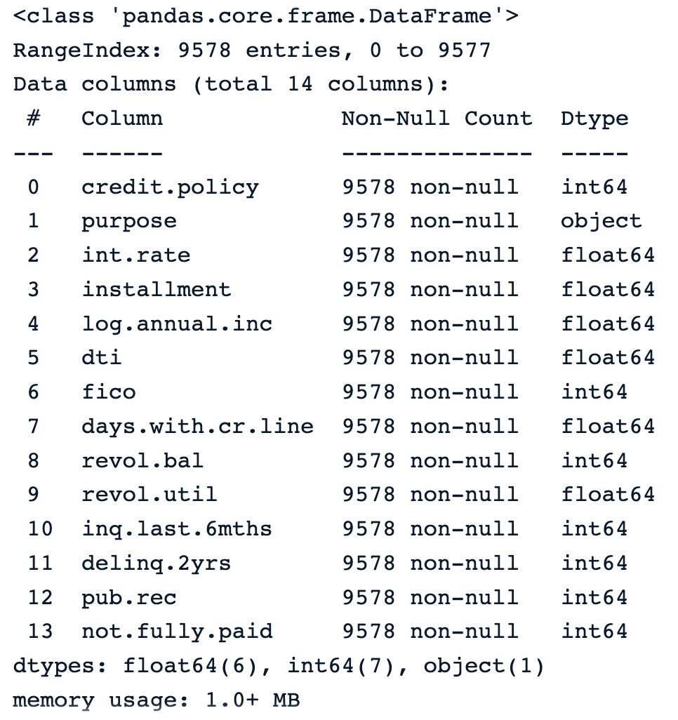

We notice an imbalanced data scenario, where there are many more observations with class 0 (8045 observations) than there are for class 1 (only 1533 observations).

print(loan_data['not.fully.paid'].value_counts())
loan_data['not.fully.paid'].value_counts().plot(kind='barh')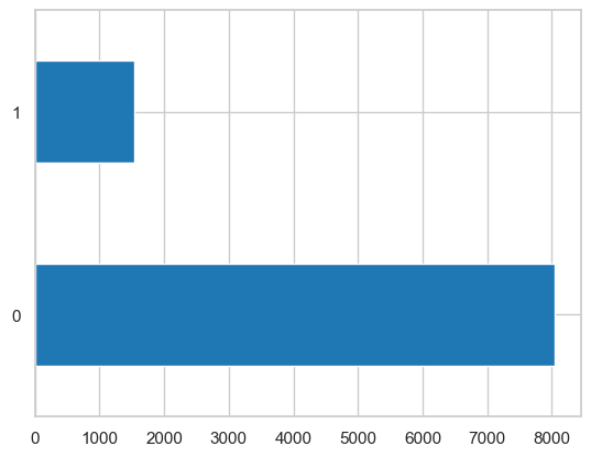

Using such imbalanced data for model training affects the overall performance. 

One way of tackling this issue is using the undersampling approach, meaning we are reducing the number of the majority observations (class 0). In this scenario, there will be as many observations for class 0 as there are for class 1, and the process is as follows:

• First get the number of class 1.

• Select N random observations from class 0, where N is the size of the dataframe of class 1.

• Concatenate the previous two dataframes.

loan_data_class_1 = loan_data[loan_data['not.fully.paid'] == 1]
number_class_1 = len(loan_data_class_1)
loan_data_class_0 = loan_data[loan_data['not.fully.paid'] == 0].sample(number_class_1)

final_loan_data = pd.concat([loan_data_class_1,
                         	loan_data_class_0])

print(final_loan_data.shape)

The Diving Deep with Imbalanced Data tutorial provides more resources to learn the techniques to deal with an imbalance dataset. 

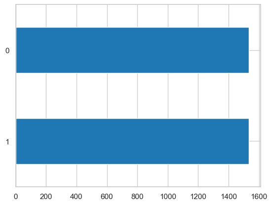
After the undersampling, we get: 

• Overall 3066 observations and 14 columns. 

And the final balanced distribution is shown below.

Prepare the data for training 

By looking at the data set, we notice that not all the features have the same scale, and some machine learning models such as KNN are sensitive to such a scaling. This issue can be addressed by normalizing the ranges of the features to the same scale using the MinMaxScaler module. In this case, between 0 and 1.

Also, we will remove the purpose column for simplicity’s sake since it requires additional preprocessing. 

from sklearn.preprocessing import MinMaxScaler

scaler = MinMaxScaler(feature_range=(0, 1))

# Remove unwanted 'purpose' column and get the data
final_loan_data.drop('purpose', axis=1, inplace=True)
X = final_loan_data.drop('not.fully.paid', axis=1)

normalized_X = scaler.fit_transform(X)

Like in any predictive task, we need to split the data into training and testing sets. In this case, we will use 77% for training and the remaining 33% for testing.  

• Random state attribute is initialized with a random value (2023 in our case) to ensure the reproducibility of the results. 

Stratify is used to ensure that the y target value is evenly distributed in both training and testing data.

from sklearn.model_selection import train_test_split

y = final_loan_data['not.fully.paid']
r_state = 2023
t_size = 0.33

X_train, X_test, y_train, y_test = train_test_split(normalized_X, y,
                                                	test_size=t_size,
                                                	random_state=r_state,
                                                	stratify=y)

All the models will follow the sequence of training on the training data, make the prediction on the testing data and evaluate the models’ performance. 

Bagging model 

Random Forest is the bagging model used in this section. We will use the default parameters for simplicity.

from sklearn.ensemble import RandomForestClassifier
from sklearn.model_selection import cross_val_score

# Define the model
random_forest_model = RandomForestClassifier()
# Fit the random search object to the data
random_forest_model.fit(X_train, y_train)

After training the model, the performance is generated using the accuracy_score function as follows: 

# Make predictions
y_pred = random_forest_model.predict(X_test)

# Get the performance
accuracy = accuracy_score(y_test, y_pred)

print("Accuracy:", accuracy) 

The previous print statement generates 0.6156 which is 61.56%

Now let's compare this score to the performance of a blending aggregation approach.

Blending Model 

For blending, we will use two base models: a decision tree and a K-Nearest Neighbors classifier. A final regression model is used to make the final predictions.

from sklearn.neighbors import KNeighborsClassifier
from sklearn.tree import DecisionTreeClassifier
from sklearn.linear_model import LogisticRegression

The original training data is split into a new training data set and a validation data set. The base models are trained on the training data. 

X_train, X_val, y_train, y_val = train_test_split(
                                            	X_train, y_train,
                                            	test_size=t_size,
                                            	random_state=r_state)

Two dataframes are then generated from the predictions of those base models: 

• First dataframe  with the predictions on the validation data concatenated with the original validation data.
• Second dataframe with the predictions on the test data concatenated with the original test data.

# Decision Tree Model
dt_model = DecisionTreeClassifier()
dt_model.fit(X_train, y_train)
dt_model_pred_val = dt_model.predict(X_val)
dt_model_pred_test= dt_model.predict(X_test)

dt_model_pred_val = pd.DataFrame(dt_model_pred_val)
dt_model_pred_test = pd.DataFrame(dt_model_pred_test)

# KNN Model
knn_model = KNeighborsClassifier()
knn_model.fit(X_train,y_train)
knn_model_pred_val = knn_model.predict(X_val)
knn_model_pred_test = knn_model.predict(X_test)

knn_model_pred_val = pd.DataFrame(knn_model_pred_val)
knn_model_pred_test = pd.DataFrame(knn_model_pred_test)

The final logistic regression model is built using the concatenated validation data, and evaluated using the concatenated test data. 

x_val = pd.DataFrame(X_val)
x_test = pd.DataFrame(X_test)

df_val_lr = pd.concat([x_val, knn_model_pred_val,
                    	dt_model_pred_val], axis=1)

df_test_lr = pd.concat([x_test, dt_model_pred_test,
                     	knn_model_pred_test],axis=1)

# Logistic Regression Model
lr_model = LogisticRegression()

lr_model.fit(df_val_lr,y_val)
lr_model.score(df_test_lr,y_test)

Using the .score() function computes the accuracy score by default and does not need actual predictions. 

The performance result is 0.6383, which is 63.83% and is around 2% higher than the initial random forest; hence the blending model provides the best performance.

Our course Ensemble Methods in Python and Machine Learning with Tree-Based Models in R could be a great next step to continue your machine learning journey by diving into the wonderful world of ensemble classifier methods, respectively in Python and R.

Conclusion

This article has covered different types of ensemble modeling along with their features, advantages and their disadvantages. Also, it provided a brief overview of some examples of ensemble model-based algorithms such as Random Forest, Adaboost, XGBoost, Gradient Boosting Trees, and Gradient Boosting machines. 

When building ensemble models, it is important to be aware of their pros and cons for better business insights.

FAQs

What is the difference between homogeneous and heterogeneous learners?

Homogeneous learners are learners with a similar type of algorithm and hyperparameters. Random forest can be considered to be an ensemble of homogeneous learners. 

Heterogeneous ones, on the other hand, have different algorithms and hyperparameters. Random forest, neural network, and KNN can be heterogeneous learners of an ensemble model.

What are the advantages of ensemble models over single models?

Using ensemble models can make better predictions over a single model.

What is the limitation of ensembling models?

Ensemble models can suffer from a lack of interpretability, meaning that the knowledge learned by the ensemble models is not understandable by end users.

When should you avoid using ensemble models?

The use of ensemble models should be avoided in the following conditions but not limited to: high interpretability,  limited data, real-time constraint, and high computation cost.  

What are the different types of ensemble methods in machine learning?

Bagging, boosting, stacking, voting, blending, and cascading are the main types of ensemble methods in machine learning.