Binomial Distribution: A Complete Guide with Examples

What is a Binomial Distribution?

A binomial distribution is a discrete probability distribution that models the count of successes in a set number of independent trials. Each trial in this scenario has only two possible outcomes, often labeled as "success" and "failure," with a consistent probability of success across all trials.

Key features of a binomial distribution include:

• A fixed number of trials n
• Independent trials
• Constant probability of success p for each trial
• Binary outcomes for each trial (success/failure)

The binomial distribution's importance in statistics stems from its ability to model real-world scenarios where we're interested in the frequency of a specific event occurring within a defined number of attempts. 

Properties of Binomial Distributions

Understanding the properties of binomial distributions is key to their effective use in statistical analysis. Let's examine some essential characteristics:

Fixed number of trials

Two parameters define a binomial distribution:

1. n: The set number of independent trials
2. p: The probability of success in each trial

These parameters determine the shape and features of the distribution. The fixed trial count distinguishes binomial distributions from related concepts like the Poisson distribution, where event counts can fluctuate.

In statistical modeling, these parameters have some important implications. The fixed n allows for precise probability calculations in scenarios with a known number of attempts, such as quality control inspections or clinical trials. The constant p across trials enables the modeling of consistent processes, though it may limit applicability in situations where the probability of success varies.

Mean and variance

For a binomial distribution, the mean (μ) and variance (σ^²) are calculated as:

• Mean = np
• Variance = np(1-p)

The mean represents the expected number of successes in n trials. For instance, if you flip a fair coin 100 times (n = 100, p = 0.5), you expect 50 heads on average.

The variance quantifies the spread of the distribution around the mean. A larger variance indicates greater variability in the number of successes from one set of trials to another. This measure is useful for assessing the reliability of estimates and constructing confidence intervals.

Symmetry and skewness

The parameters of a binomial distribution influence its shape:

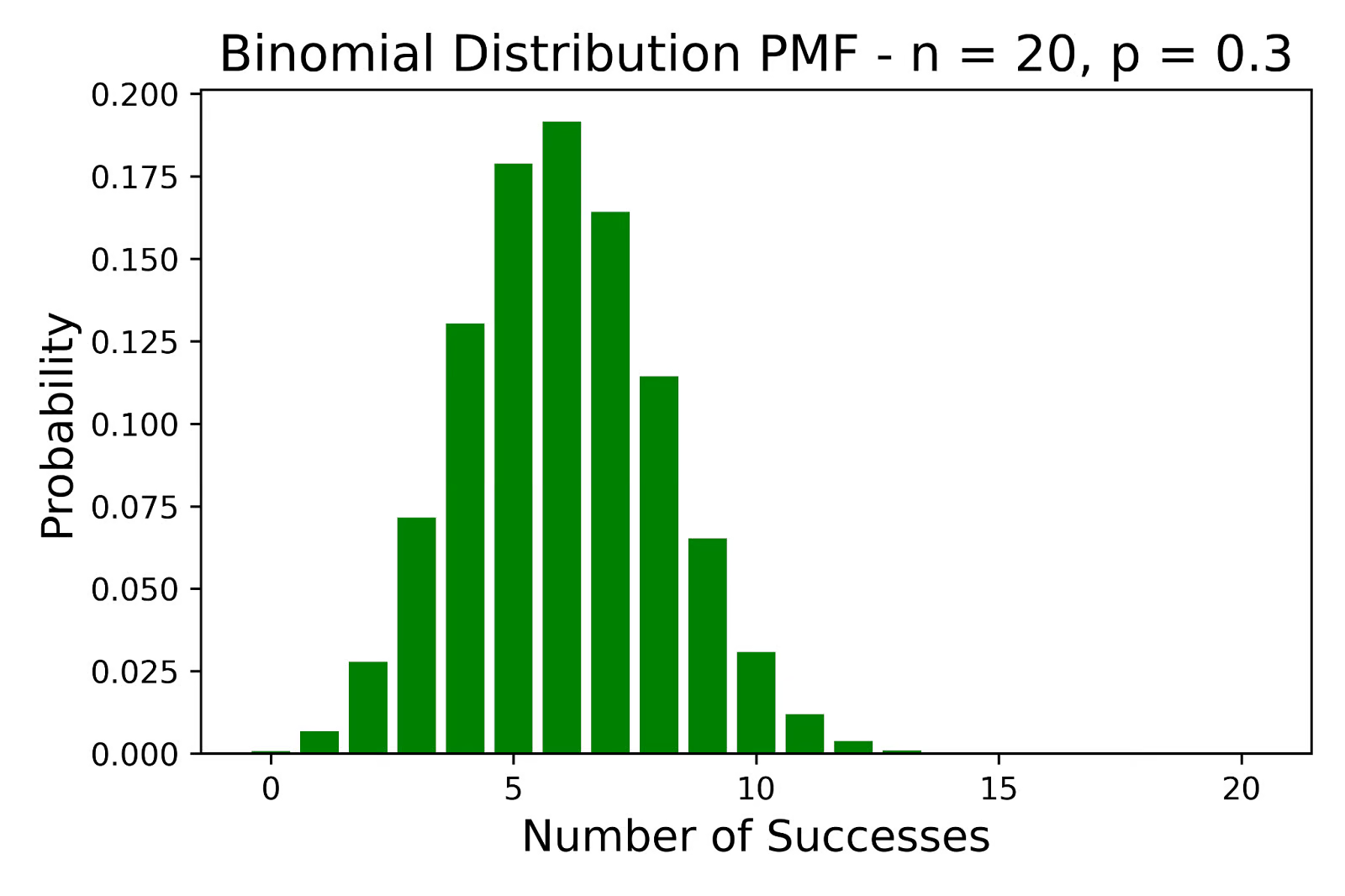
Binomial Distribution PMF - n=20, p=0.3. Image by Author.

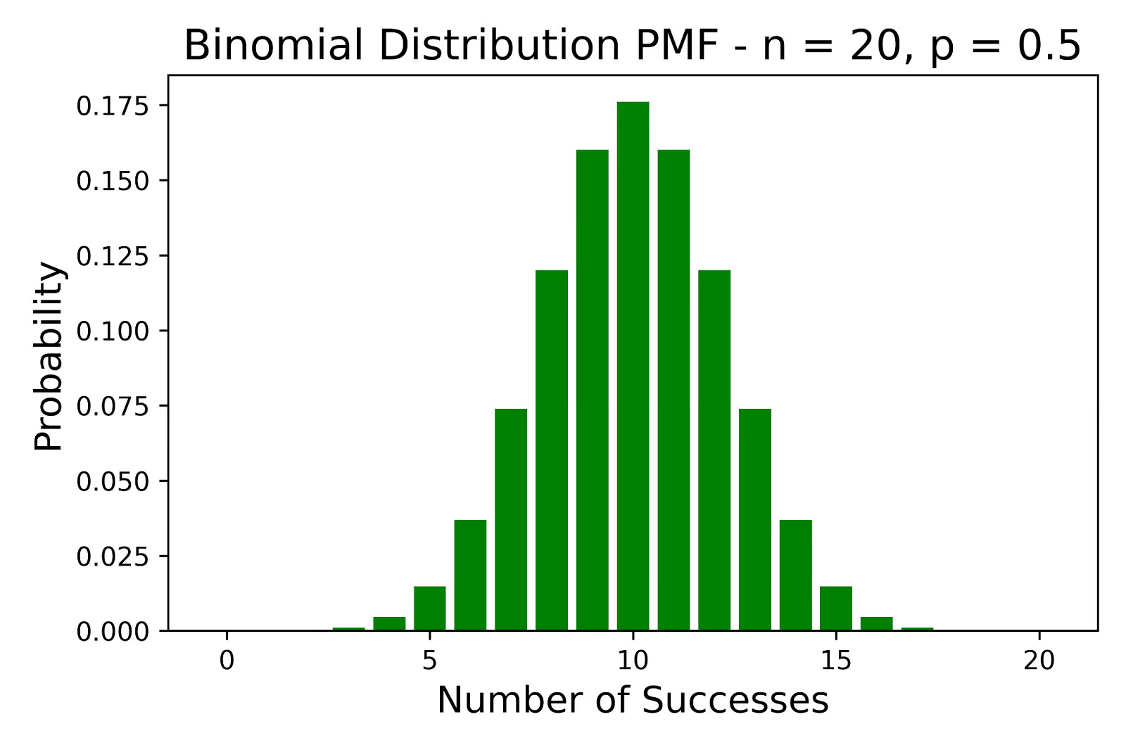
Binomial Distribution PMF - n=20, p=0.5. Image by Author.

Binomial Distribution PMF - n=20, p=0.7. Image by Author.

The above figures illustrates how the probability of success p affects the shape of a binomial distribution when the number of trials n is fixed.

• When p = 0.5, the distribution is symmetric.
• When p < 0.5, the distribution shows a positive skew.
• When p > 0.5, the distribution exhibits a negative skew.

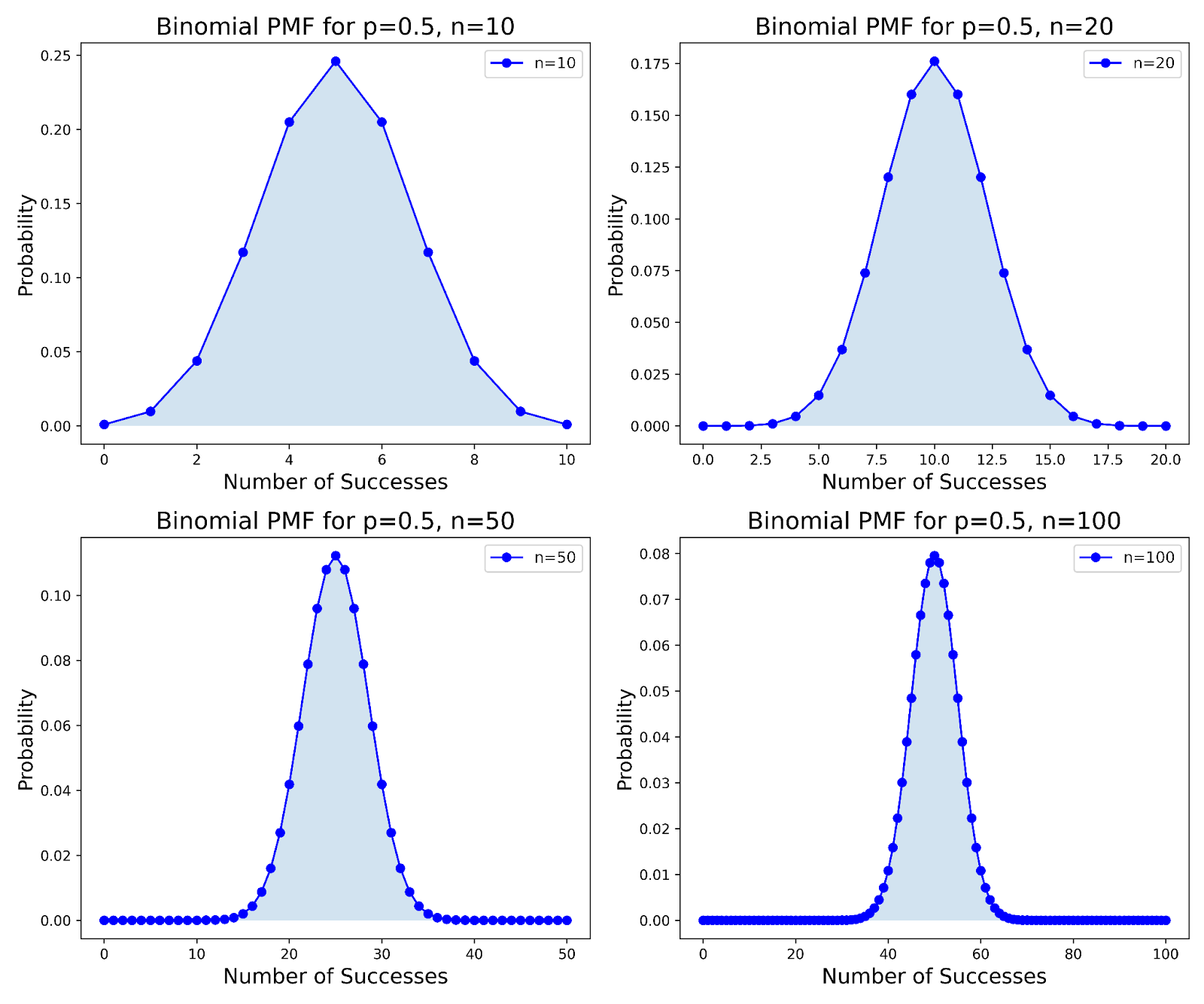
The number of trials, denoted as n, influences the shape of the binomial distribution. As n increases, the distribution progressively adopts a more bell-shaped curve. This change occurs irrespective of the probability of success p. Concurrently, the relative spread of the distribution, measured by the coefficient of variation, diminishes. Furthermore, the distribution's skewness decreases, leading to increased symmetry.

See the figure below for a visual representation of how increasing n influences the binomial distribution's shape across different trials:

Binomial PMF Comparisons for p=0.5 with Varying n Values. Image by Author.

This transformation towards greater symmetry and a bell-shaped curve aligns with the Central Limit Theorem (CLT). According to CLT, as n increases indefinitely, the binomial distribution increasingly approximates a normal distribution. This approximation holds particularly true when the product of the number of trials and the probability of success (np) and the product of the number of trials and the probability of failure (n(1−p)) are both sufficiently large.

Practical Applications of Binomial Distributions

The versatility of binomial distributions makes them applicable across many fields, particularly in scenarios involving binary outcomes.

Quality control and reliability testing

In manufacturing and quality assurance, binomial distributions help model defective item counts in production batches. For example, given the probability of a product defect and a specific inspection quantity, the binomial distribution can calculate the likelihood of finding a certain number of faulty items. This helps in making informed decisions about process improvements and quality control measures.

Survey sampling

Researchers often employ binomial distributions to model respondent counts with specific characteristics in surveys. This approach is particularly useful for yes/no questions or when categorizing responses into two groups. It assists in estimating and analyzing population proportions based on sample data.

Financial modeling

Binomial distributions are integral to certain option pricing models in finance. The binomial option pricing model uses a discrete-time framework to value options, where the underlying asset can move up or down with specific probabilities at each time step. This model provides a simplified yet effective method for estimating the potential future prices of options based on probabilistic scenarios. Our Financial Modeling in Excel course is a great resource to explore similar financial modeling concepts. 

Binomial distributions are commonly used in data analysis, but they come with specific performance considerations, especially when dealing with large values of n (number of trials) or extreme probabilities p. Understanding these factors will be helpful for effective application and interpretation of results.

Computational challenges with large n

As the number of trials n in a binomial distribution increases, several computational challenges can arise:

1. Precision Issues: Calculating exact probabilities for large n can lead to precision errors due to limitations in floating-point arithmetic.
2. Computational Intensity: Direct calculation of probabilities using the binomial probability mass function becomes computationally expensive for large n.
3. Memory Constraints: Storing all possible outcomes for large n can exceed available memory, especially in resource-constrained environments.

To manage these challenges, several strategies can be used:

1. Normal Approximation: For large n, the binomial distribution can often be approximated by a normal distribution, especially when p is not too close to 0 or 1 to avoid skewness. This approximation is considered reasonable when both np and n(1−p) are greater than 5, with more conservative estimates using a threshold of 10.
2. Poisson Approximation: When n is large and p is small but np remains moderate (typically up to about 10), the Poisson distribution provides a good approximation. This method is less computationally intensive and is particularly effective for modeling the occurrence of rare events.
3. Recursive Methods: For exact calculations, recursive algorithms can be more efficient than direct computation of combinations. These methods leverage the relationship between successive terms in the binomial probability mass function. For instance, the probability of k+1 successes can be computed from the probability of k successes using a simple multiplicative factor. This approach can significantly reduce computational time, especially for large n.
4. Logarithmic Transformations: Working with logarithms of probabilities can help avoid underflow and overflow issues in computations, particularly when dealing with very large n or extreme values of p. This technique involves summing logarithms instead of multiplying probabilities, which can preserve numerical precision. It's especially useful when computing likelihood ratios or working with products of probabilities.

Dealing with small probabilities

When working with very small success probabilities (p), several implications arise:

1. Skewness: The binomial distribution becomes highly right-skewed, making it challenging to interpret and work with standard symmetric measures.
2. Spread: The variance of the distribution becomes very small relative to the mean, which can lead to numerical instability in some calculations.
3. Rare Event Modeling: Small probabilities often correspond to rare events, which can be challenging to model accurately.

Techniques for handling these situations include:

1. Poisson Approximation: As mentioned earlier, the Poisson distribution can provide a good approximation when p is small and n is large.
2. Negative Binomial Modeling: Instead of modeling the number of successes in a fixed number of trials, it might be more appropriate to model the number of trials until a fixed number of successes occurs.
3. Logarithmic Transformations: Working on a logarithmic scale can help manage the numerical challenges associated with very small probabilities.
4. Importance Sampling: In simulation studies, techniques like importance sampling can be used to more efficiently estimate rare event probabilities.

Common Misconceptions

To effectively utilize binomial distributions, it's important to address some frequent misunderstandings:

Distinguishing from Bernoulli distribution

While related, the Bernoulli and binomial distributions are distinct. A Bernoulli distribution models a single trial with two possible outcomes, whereas a binomial distribution tracks success counts across multiple trials. A binomial distribution with n=1 is equivalent to a Bernoulli distribution.

Interpreting the number of trials

It's essential to remember that in a binomial distribution, the trial count n must be fixed and known beforehand. If the number of trials can vary, alternative distributions like the negative binomial distribution might be more suitable.

Alternatives to Binomial Distributions

While binomial distributions are versatile and widely applicable, certain situations may call for alternative distributions. Understanding these alternatives can provide data scientists and statisticians with a broader toolkit for modeling various scenarios.

Poisson distribution

The Poisson distribution is a discrete probability distribution that expresses the probability of a given number of events occurring in a fixed interval of time or space, assuming these events occur with a known constant mean rate and independently of the time since the last event.

Key characteristics of the Poisson distribution:

• It models the number of events in a fixed interval.
• It assumes events occur independently.
• It is defined by a single parameter λ, which is both the mean and variance of the distribution.

The Poisson distribution serves as an effective alternative to the binomial distribution in cases where:

• The number of trials n is large.
• The probability of success p is small.
• The product np is moderate (typically less than 10).

A few scenarios where the Poisson distribution could be a better fit than a binomial distribution include: 

• Quality Control: For instance, monitoring the number of defects in a large manufacturing process where each individual item has a small chance of being defective.
• Customer Traffic Analysis: Estimating the number of customers visiting a store each hour, where visits are considered independent from one another.
• Environmental Monitoring: Counting the frequency of certain natural phenomena, such as radioactive emissions over a given time frame, where the occurrences are discrete and independently timed.

In these applications, the Poisson distribution provides a powerful tool for data analysis, particularly in conditions where the binomial distribution’s computations become cumbersome or less precise. 

Negative binomial distribution

The negative binomial distribution is another discrete probability distribution that provides an alternative modeling approach to the binomial distribution in certain scenarios.

Key characteristics of the negative binomial distribution:

• It models the number of failures before a specified number of successes occurs.
• It is defined by two parameters: the number of successes required r and the probability of success on each trial p.

The negative binomial distribution differs from the binomial distribution in a fundamental way:

• Binomial: Models the number of successes in a fixed number of trials.
• Negative Binomial: Models the number of trials needed to achieve a fixed number of successes.

This distribution is particularly useful in scenarios where:

• The process continues until a predetermined number of successes is reached.
• The number of trials is not fixed in advance.
• There's a need to model over-dispersed count data. Over-dispersion occurs when the observed variance in data is greater than what the model (usually assuming a binomial distribution) expects.

A few scenarios where the negative binomial distribution could be a better fit than a binomial distribution include:

• Sales Process Modeling: For instance, tracking the number of sales calls required to achieve a target number of successful sales, where the process continues until the target is reached.
• Insurance Risk Assessment: Analyzing the number of claims filed before a certain number of large claims occur, which is crucial in actuarial sciences for pricing policies and managing risk.
• Ecological Studies: Modeling capture-recapture scenarios in wildlife populations, where researchers continue sampling until a predetermined number of tagged animals are recaptured.

In these applications, the negative binomial distribution provides a flexible tool for data analysis, particularly in situations where the endpoint is defined by a number of successes rather than a fixed number of trials.

Conclusion

Keep in mind that while the binomial distribution is a fundamental concept, it's just one of many statistical methods available. Keep looking at related concepts like the Poisson and negative binomial distributions to further enhance your analytical capabilities.

To deepen your understanding of binomial distributions and related statistical concepts, consider exploring these resources:

• For a solid foundation in statistics, our Introduction to Statistics course covers essential concepts, including probability distributions.
• If you're working with Python, the Foundations of Probability in Python course and Introduction to Statistics in Python course offer hands-on practice with statistical concepts and their implementation.
• For R users, the Introduction to Statistics in R course provides a comprehensive introduction to statistical analysis using R.

By continuing to build your statistical knowledge and skills, you'll be well-prepared to tackle complex data analysis challenges across various domains. As a last thing, make sure to click below to become a machine learning scientist today.