Excel Drop Down List: Setup, Tips, and Troubleshooting

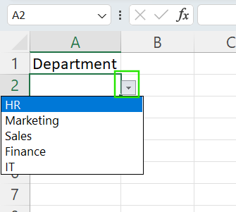
Have you ever clicked on a little arrow in an Excel cell and it displays a list of options? This could be a list of departments, regions, statuses, or categories. If you answer yes, you’ve interacted with a drop-down list. 

Excel drop-down lists guide users toward consistent input, reducing the chances of typos or mismatched entries. Whether filling out a project tracker, creating a budgeting sheet, or designing a form that others will use, drop-downs help keep things neat and predictable.

In this guide, I will show you how to create these lists from scratch, customize them to fit your needs, fix them when things go wrong, and even build more dynamic and interactive versions for advanced workflows. You don’t need to be an Excel expert to get started; just a working spreadsheet and a few data points are enough. 

If you are getting started in Excel, our Introduction to Excel course covers skills like navigating the interface, understanding data formats, and working with basic functions. Also, I find the Excel Formulas Cheat Sheet, which you can download, is a helpful reference because it has all the most common Excel functions.

Creating Basic Drop-Down Lists in Excel

Now, let’s look at how you can create a drop-down list in Excel

Step-by-step construction

To construct a drop-down list in Excel, use these steps:

Step 1: Prepare the source data

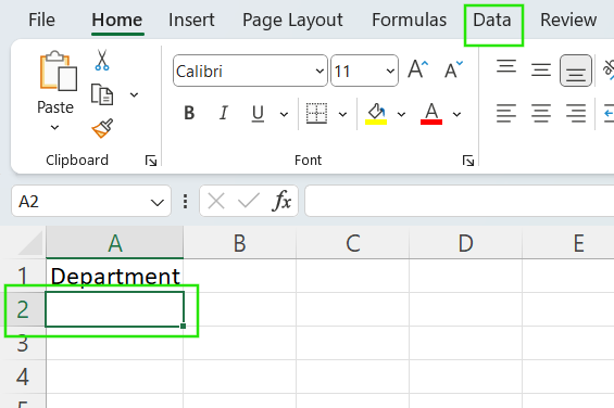
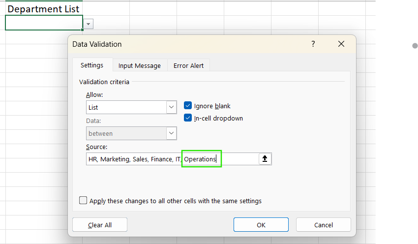
Before you create a drop-down, decide on what items to include in the list. You can type these choices directly when setting up the drop-down, or list them in cells in your spreadsheet.

Step 2: Applying data validation

When your list is ready:

• Highlight the cell or range of cells where you want the drop-down to appear.

• Go to the Data tab on the ribbon and click Data Validation.

• In the dialog box that appears, under Allow, choose List.

• In the Source box, type your values directly or reference the cell range where your list is located.

Step 3: Finalizing and testing

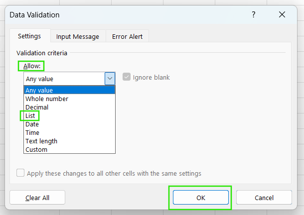
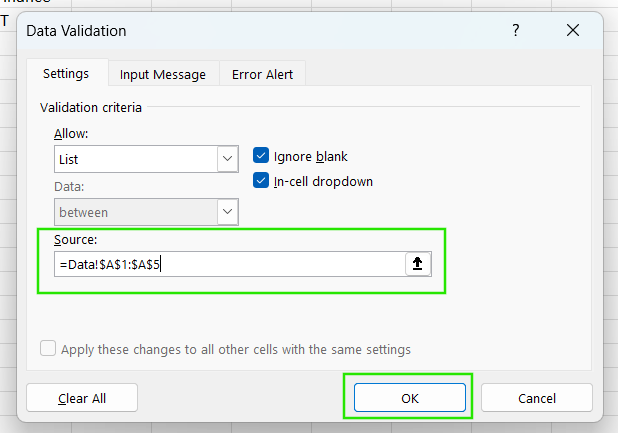
After verifying you have entered the correct range:

• Press OK to finish.
• Click into one of the validated cells. You will see a small arrow on its right, where you can select your entry from the list.

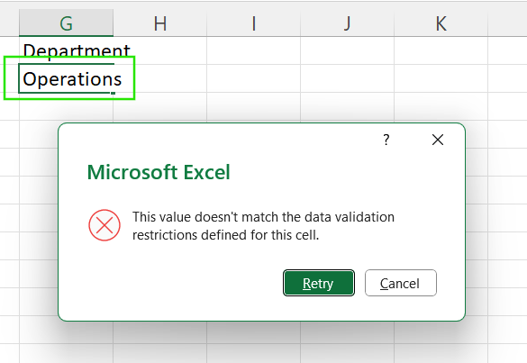
If you manually input an item that you had not predefined into the cell, you will get an error. This validation helps prevent errors during data entry.

Table-based dynamic lists (Table Magic)

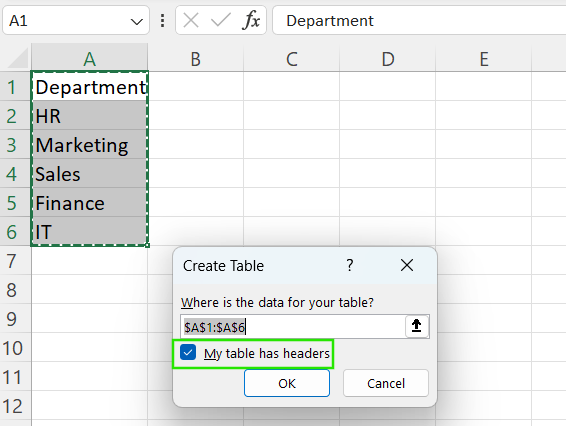
If you need more control of your lists, you can use Excel tables to create dynamic lists. Follow the steps below:

• Select your source list and press Ctrl + T (or go to the Insert tab > Table).
• Make sure to check “My table has headers”.

• Give your table a meaningful name under the Table Design tab.

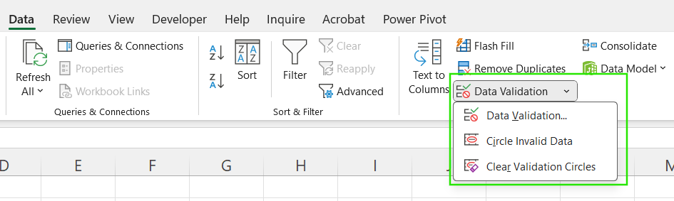
• Select the cell range where your drop-down list should appear, then select the Data tab > Data Validation > List.

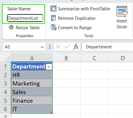
• In the “Source” field, type =INDIRECT("DepartmentList[Department]")

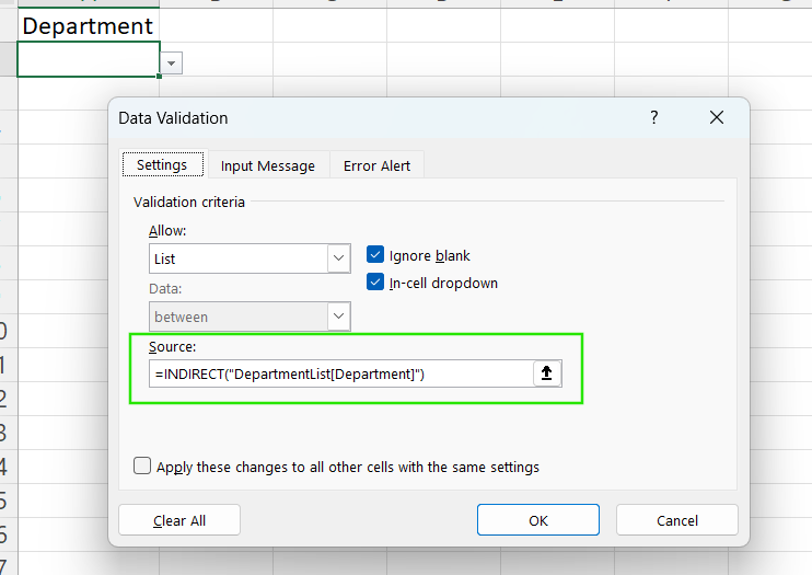
When you convert your source list into a table, you allow Excel to automatically include new items in the drop-down list as they are added. 

Check out the Excel Shortcuts Cheat Sheet to learn how to improve productivity by learning the shortcuts for different Excel features.

How to Add or Remove Items from a Drop-Down List

At some point, you may need to update your drop-down list. I will show you how to remove or add items to the drop-down list.

If you created your drop-down list using manual input, simply add the new item at the end of the list.

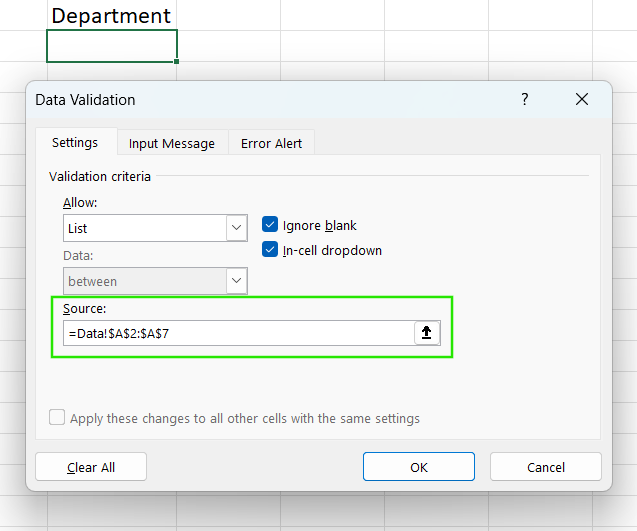
You can also add the new item to your cell range if you selected the “Source” as a cell-range.

If you are referencing your list from an Excel table (like the one I showed earlier), type the new value below the last row. Excel will automatically extend and update the table, which will also update your list.

How to Remove a Drop-Down List

You can remove a drop-down list from your Excel sheet without deleting the data you have already entered.

To remove a drop-down list created using Data Validation:

• Select the cell or range containing the drop-down.
• Go to the Data > Data Validation.
• In the dialog box, click Clear All > OK.

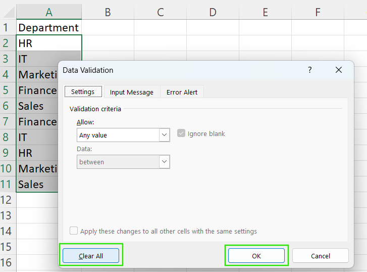
This method removes the validation rule and the drop-down arrow. The existing cell values remain intact but are no longer restricted to the previous drop-down options.

If you are using combo boxes or ActiveX controls:

• Go to the Developer > Design Mode.
• Select the control, then press Delete on your keyboard.

You should note that your existing data will remain intact even after removing the validation rules for the drop-down list.

Advanced Techniques: Dynamic and Dependent Lists

Now that you have learned the basics of Excel drop-down lists, let’s see how you can create flexible lists for advanced uses.

Dynamic drop-down lists

Dynamic drop-down lists update automatically whenever you change the source data. If your list has duplicates, it’s a good idea first to use the UNIQUE() function to pull out the distinct values. For example, if your data is in “A2:A21”, you can use the formula below in another spot to create a cleaner list for your drop-down.

=UNIQUE(A2:A21)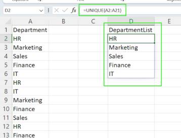

Then you can use this output range as the source for your drop-down.

You can also use the OFFSET() function if your list grows, but you don’t want to convert it into a formal table. 

=OFFSET(ListData!$A$2, 0, 0, COUNTA(ListData!$A:$A) -1)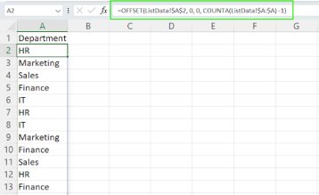

The dynamic drop-down lists are used in live forms, tracking sheets, or collaborative spreadsheets. This feature ensures automatic updates as users enter data or when data changes.

Dependent (cascading) drop-downs

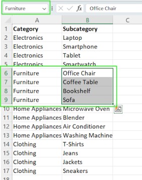
Dependent drop-down lists (cascading drop-down lists) are sets of drop-downs where the choices in one list depend on the selection made in another. These are ideal for hierarchical data like categories and subcategories.

When creating the dependent drop-down lists, you first create named ranges for each sub-item group. The second drop-down uses the INDIRECT() function to reference the named range corresponding to the first selection.

Step 1: Prepare your source data

Create a list of categories and sub-categories in separate columns following a particular sequence. Ensure that each sub-category range is named using the appropriate “Category” name as it appears in the list.

Step 2: Create the first drop-down list

In the first drop-down menu, select the main category range. Use Data Validation > List and set the source from the ‘Category’ column range. This step should be similar to the one we have used before.

Step 3: Create the dependent drop-down list

Next, set up the sub-category drop-down. Go to Data Validation > List. For the source, point it to reference the cell on the first drop-down list.

=INDIRECT(A2)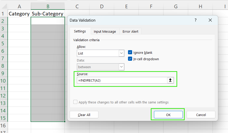

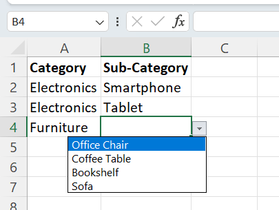
Step 4: Test the drop-down

Check if the items are correctly placed in the ‘Category’ and ‘Sub-Category’ columns.

The following are common issues to look out for when using dependent drop-down lists:

• Ensure the named subcategory ranges match the text in the main category drop-down. You should have no extra spaces and match the case.

• If INDIRECT() returns a #REF! error, double-check that the named ranges exist and correspond to the main list values.

Customization and User Experience

You can make your drop-down lists more flexible to enhance user experience and improve usability. In this section, I will show you how to customize the drop-down lists for different use cases.

Input messages and error alerts

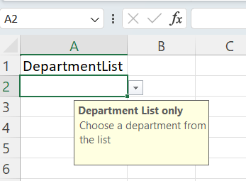
Excel lets you attach short messages to drop-down cells to help users make the right selection. To set up an input message:

• Select the drop-down cell.
• Go to Data > Data Validation.
• Switch to the Input Message tab.
• Enter a title and message like “Choose a department from the list.”

The drop-down arrow will appear with a message next to the selected cell. This will help the user understand the data required for the field.

You can create “Error” alerts appear if someone tries to enter data that doesn’t match the drop-down options. To customize this feature:

• Go to Data Validation > Error Alert tab.
• Choose the alert style: Stop (prevents invalid data entry), Warning (warns but allows override), or Information (shows info but lets entry proceed)
• Provide a message explaining the restriction, such as “Please select a valid department from the list.”

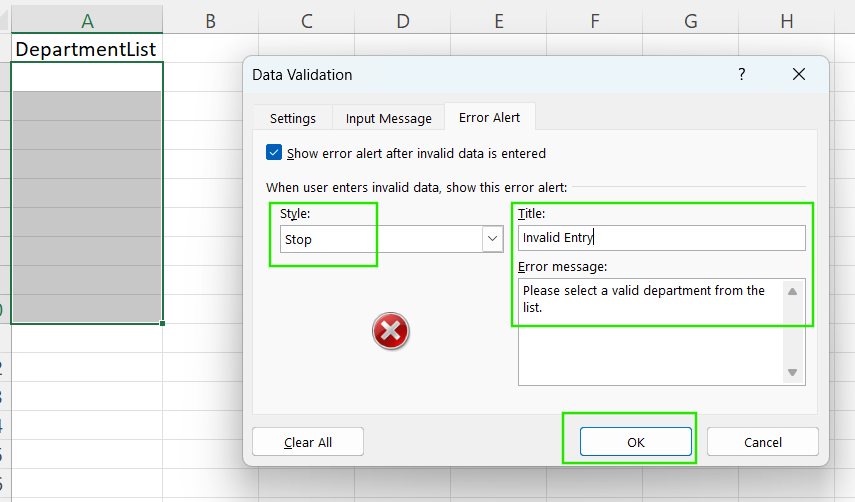
Always use clear, user-friendly language in both input messages and error alerts to improve the clarity of the messages.

Searchable drop-downs

In modern Excel versions, such as Microsoft 365 and Excel for the web, you can use searchable drop-down functionality, especially when navigating a long list of items. When you click the drop-down arrow, you can start typing, and Excel filters the list to match your input. This feature is important when working with long lists, such as customer names, product SKUs, or country names.

However, searchable drop-downs are only available in recent Excel versions and not in older desktop versions like Excel 2016 or 2019. If you are using the older Excel versions, use combo boxes or form controls with built-in search capabilities via VBA to create searchable drop-down lists.

Allowing other entries or manual input

Sometimes you might want to add items to your list while bypassing the original validation. If you want to add custom data:

• Select the cell or range of cells where you want the drop-down to appear.
• Go to Data > Data Validation.
• On the Error Alert tab, uncheck the “Show error alert after invalid data is entered” box.

When you uncheck this option, you can enter any value that is not in the drop-down options list.

While enabling manual entry increases flexibility, it can lead to inconsistent or invalid data if users mistype or enter unexpected values. It also reduces the benefit of having a controlled list.

To handle such unlisted entries:

• Use conditional formatting to flag cells with values not in the validated list for review.

• Create helper columns that check validity. For example, use COUNTIF() to verify if the entry exists in the source list.

• Regularly audit and update your source lists to accommodate valid new entries.

Check out our Conditional Formatting in Google Sheets course to learn how to apply conditional formatting to validate data for getting quick insights.

Form Controls and ActiveX for Enhanced Functionality

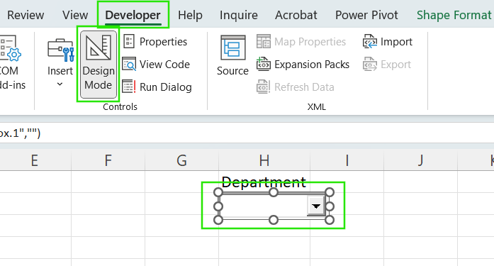
If you need even greater flexibility and functionality of your drop-down lists, Excel offers advanced controls like Form Control and ActiveX combo boxes.

Form Control combo boxes

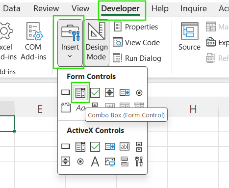
Form Control combo boxes work as the standard drop-down lists but allow users to link them with other cells. This method is useful when integrating drop-down lists with forms or dashboards.

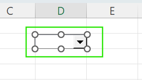
To use the combo boxes:

• Go to the Developer tab.
• Click Insert > Form Controls, choose Combo Box.

• Draw the combo box on your worksheet.

• Right-click the control and select Format Control.

• In the Control tab, set the “Input Range” and a “Cell Link” where the selected item’s index will appear.

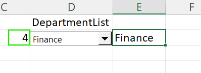
You will note that the combo box returns a number corresponding to the item’s position in the list. You can retrieve the actual value from the item’s position using the INDEX() function.

Form controls are preferred when building interactive dashboards or reports. They can also be used in scenarios where VBA isn’t necessary, but you need more flexible formatting than standard data validation allows.

ActiveX Control boxes

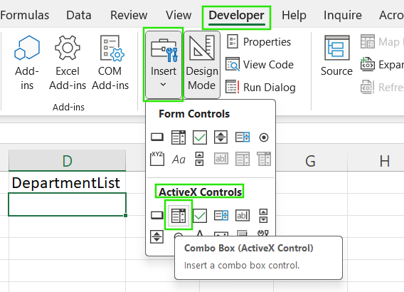
ActiveX Control boxes offer more power and customization, including font control, auto-complete, and the ability to trigger macros based on user interaction.

To add the ActiveX Control boxes

• Go to Developer tab > Insert > ActiveX Controls > Combo Box.

• Draw the box on the sheet.
• Right-click it and choose Properties to configure like “ListFillRange”, “LinkedCell”, then customize fonts, background colors, and border styles.

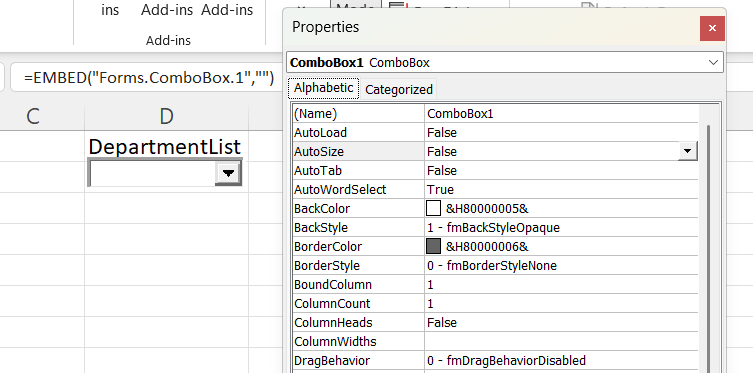
The advantage of using ActiveX Combo Box is that it offers greater formatting flexibility for fonts, colors, and layout. It also enables event-driven programming for highly interactive forms and applications. This feature Integrates with macros and automation.

However, ActiveX controls only work on Windows and are not supported in Excel for Mac or Excel Online. They are also heavier than form controls and can slow down performance in large workbooks. For advanced use, you may require some VBA knowledge.

Troubleshooting Common Issues

Even with advanced features, you may experience some issues when working with drop-down lists in Excel. Let us explore the common pitfalls and how to debug these issues.

List errors and fixes

The following are the common issues and how to fix them:

• Blank options in the drop-down: Your drop-down list may include empty or blank lines. To solve this, ensure your source range does not include blank cells.
• Missing items in the drop-down: Some items may not appear in your drop-down list. To fix this issue, verify that the source range or table includes all expected items. Confirm that the Data Validation source range covers the complete list for range-based lists and adjust as necessary.
• Incorrect or outdated references: If you have incorrect references, confirm that your Data Validation source formula or list points to the correct worksheet and cell range. Also, watch for typos or accidental changes to named ranges.
• Drop-down list not appearing or drop-down arrow missing: If you remove data validation, the drop-down list may not appear. Always ensure you have “List” as the validation type and reapply Data validation whenever you clear the formatting.

Advanced Debugging

Some of these issues may involve formula errors or spill behavior related to dynamic lists and named ranges:

• #REF! errors: This error occurs when a formula or named range refers to a deleted cell, sheet, or table. Review and update named ranges or formulas that use OFFSET(), INDIRECT(), or dynamic array functions to fix this error.

• #SPILL! errors: This error occurs when a dynamic array formula like UNIQUE() tries to output values, but other data blocks the spill area. Always check that no merged cells are empty to let the formula fill the adjacent cells.

• Dynamic array misalignment: If you create your list using functions like UNIQUE(), SORT(), or FILTER(), the output may change in size. Therefore, use a dynamic named range or refer to the whole column of the formula output.

I recommend taking our Advanced Excel Functions course to learn more about offsetting and dynamic ranges in Excel.

Conclusion

Drop-down lists in Excel are useful for guiding data entry, ensuring consistency, and enhancing the overall usability of your spreadsheets. From basic list creation and dynamic table links to cascading selections and custom form controls, these tools help make spreadsheets more interactive, accurate, and user-friendly. 

Mastering drop-down techniques reduces errors, improves data consistency, and lays the groundwork for more professional and scalable spreadsheet solutions. I encourage you to advance your skills by learning to integrate drop-down functionality with Power Query or using VBA to unlock even greater automation and intelligence in your Excel workflows.

If you want to advance your Excel skills, I recommend taking our Data Analysis in Excel course. This course will help you master advanced analytics and propel your career. I also recommend taking our Intermediate Power Query in Excel course to learn about data transformation and using the M language for creating dynamic functions.