Excel Time Formulas: Calculate, Format, and Manipulate Time in Excel

Excel makes it easy to work with numbers, but handling time (in my opinion) is a different story. The confusing part (which I’ll cover below) is that Excel stores and processes time values as fractional days, which can lead to unexpected results if you're not familiar.

In this tutorial, I will walk you through everything from creating and formatting time values to solving common problems like negative durations and time overflows. By the end, you will know how to build smarter, more reliable spreadsheets for project planning, payroll, or whatever else you are working on.

Understanding Excel’s Date System

We have to start with Excel's date system. Excel stores dates as a sequential serial numbers, starting from January 1, 1900, which is represented by the value 1. Each subequent day increases the serial number by 1. For instance:

• January 1, 1900 = 1

• January 2, 1900 = 2

• December 31, 2023 = 45205

Time values are stored as fractions of a day. For example:

• 6:00 AM = 0.25 (6 hours is 25% of a 24-hour day)

• 12:00 PM = 0.5

• 6:00 PM = 0.75

Combining dates and time is as simple as adding the two values together. For example, the formula below combines a date and time:

=A2 + TIME(10, 30, 0)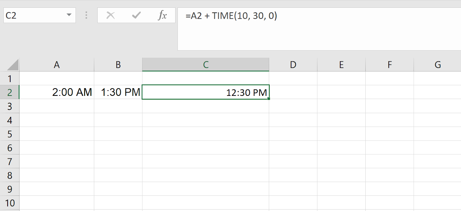

If A2 contains 45205 (December 31, 2023), the result will be 45205.4375, representing 10:30 AM on December 31, 2023.

How To Create Time Values in Excel

Let’s look at the two most common ways to create valid time values in Excel: using the TIME() function and converting text with TIMEVALUE().

Use the TIME() function

I mentioned this one earlier. The TIME() function lets you build a time value from separate components: hour, minute, and second. Here’s the syntax:

=TIME(hour, minute, second)

For example, if you want to represent 10:30 AM, you can write:

=TIME(10, 30, 0)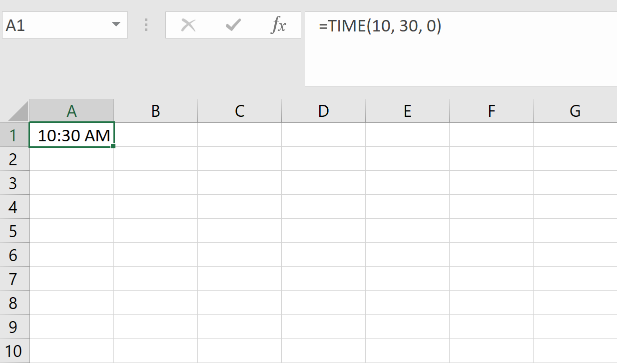

This creates a proper Excel time value for 10:30 AM, which is stored internally as 0.4375 (since 10 hours and 30 minutes is 43.75% of a 24-hour day).

Excel is flexible with the values you enter. If you exceed normal time boundaries, Excel rolls over the extra time. For instance:

=TIME(27, 0, 0)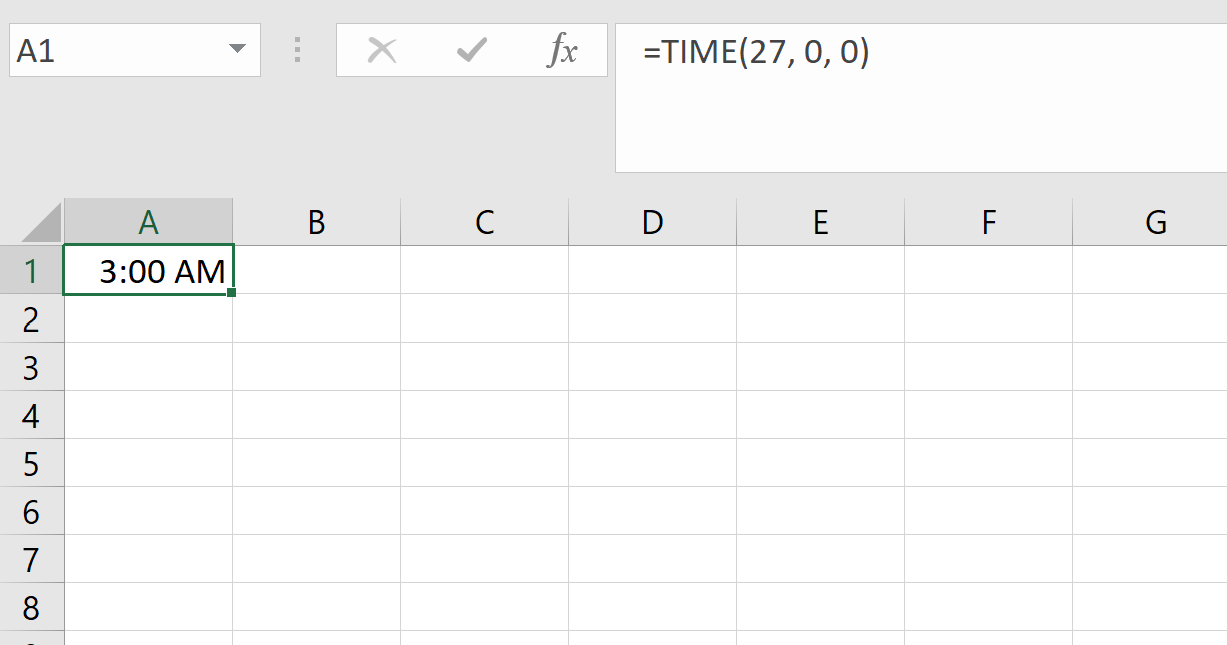

This returns 3:00 AM because 27 hours is the same as one full day (24 hours) plus 3 hours. Similarly:

=TIME(10, 75, 0)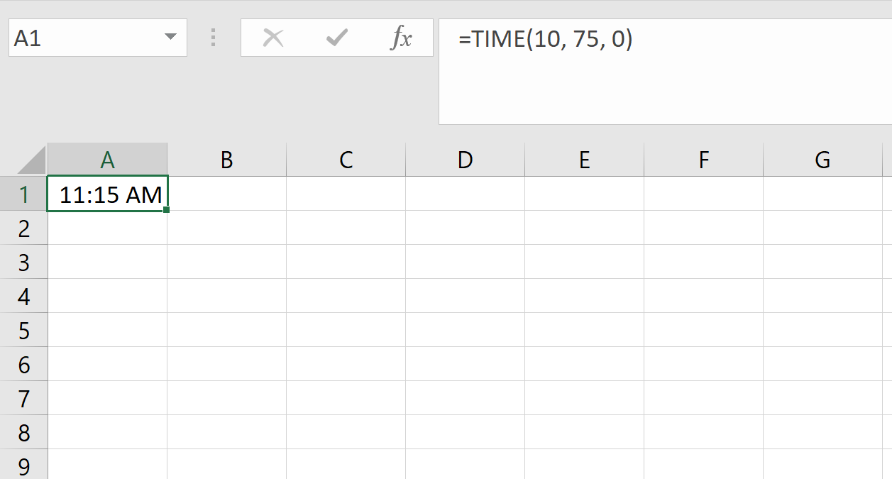

This is is interpreted as 11:15 AM, since 75 minutes becomes 1 hour and 15 minutes.

These edge cases are important to understand, especially if you are generating time values dynamically using formulas.

Use the TIMEVALUE() function

You can convert text to time with TIMEVALUE(). So if your spreadsheet includes time written as text, like “2:30 PM” or “14:45”, Excel might not treat it as a time value automatically. That is where TIMEVALUE() comes in.

=TIMEVALUE("2:30 PM")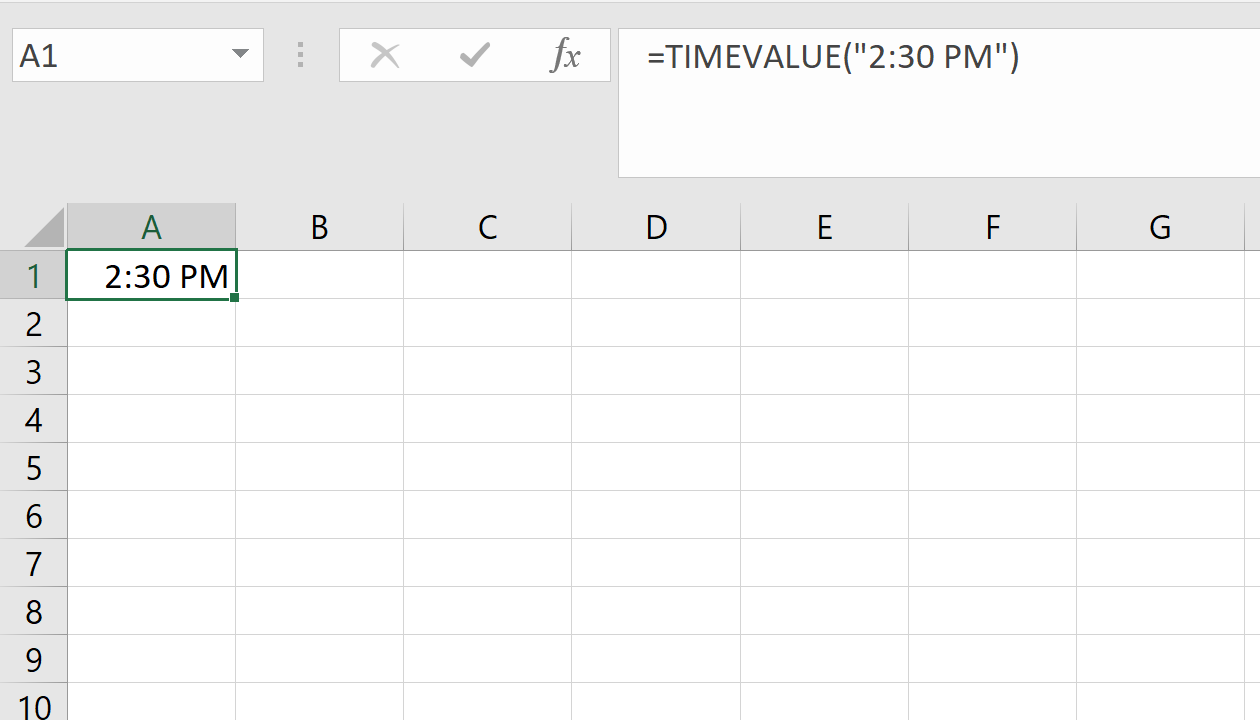

This converts the text string into an Excel time value. You can now use it in calculations just like any other time.

It is worth noting the difference between TIME() and TIMEVALUE():

• TIME() builds a time from separate numbers (hour, minute, second)

• TIMEVALUE() converts a text string into a time

Both return values that Excel recognizes as valid times, which is what you need for accurate math and formatting.

How to Calculate Time Differences

Once you have valid time values in Excel, one of the most common tasks is calculating how much time has passed between two points. Whether you are measuring the length of a shift or computing the time it takes to complete a task, Excel gives you multiple ways to get the answer.

Let’s explore the most useful approaches, from simple subtraction to more advanced tricks.

Subtract two times directly

The most straightforward way to calculate a time difference is to subtract the start time from the end time. 

For example, if cell A1 contains 10:00 AM and B1 contains 1:30 PM, the formula would look like this:

=B1 - A1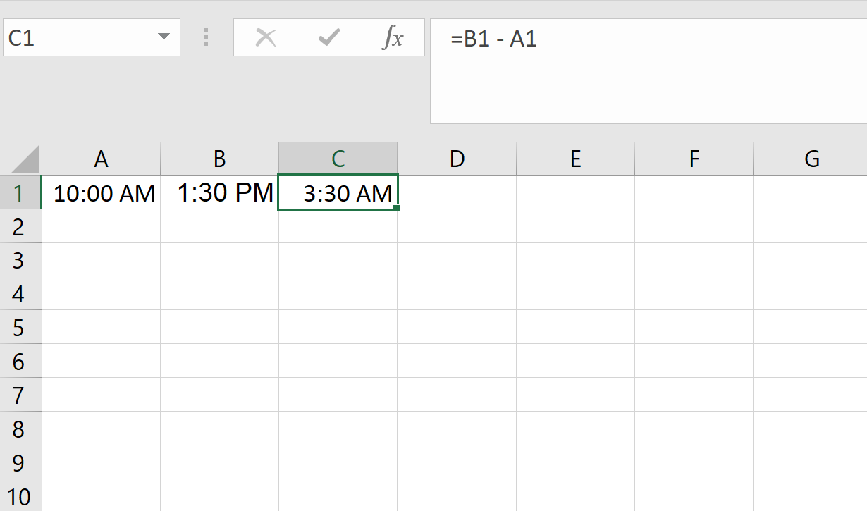

The result will be 0.145833. This might look odd at first, but remember that Excel represent time as a fraction of a day. In this case, 0.145833 equals 3 hours and 30 minutes.

To make the result more useful, you will usually want to convert it into a human-readable format.

Convert time differences to hours, minutes, or seconds

You can multiply the result of a time subtraction to express the difference in hours, minutes, or seconds. Here is how to convert a time difference to hours:

=(B2 - A2) * 24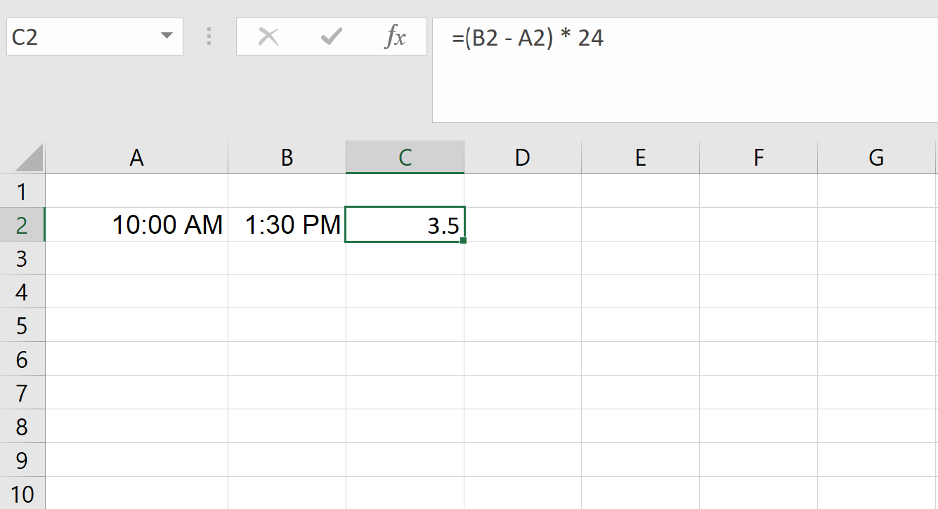

Here is how to convert a time difference to minutes:

=(B2 - A2) * 1440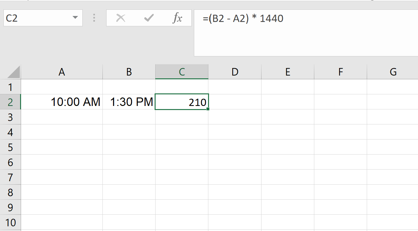

Here is how to convert a time difference to seconds:

=(B2 - A2) * 86400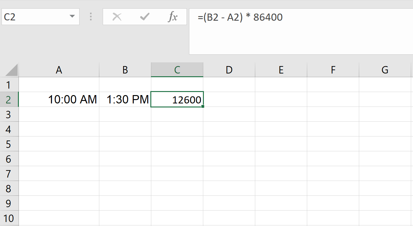

These formulas work because there are 24 hours, 1,440 minutes, and 86,400 seconds in a day. If the time difference is three and a half hours, you will get 3.5 from the hours formula, 210 from the minutes formula, and 12,600 from the seconds formula.

Extract specific time units

If you only want to pull one part of the time, say just the minutes or hours, you can use HOUR(). HOUR() returns the hour portion of a time.

=HOUR(B2 - A2)

MINUTE() returns the minute portion.

=MINUTE(B2 - A2)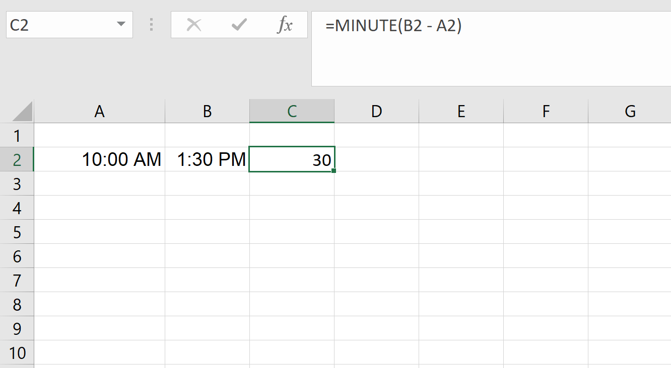

SECOND() returns the seconds.

=SECOND(B2 - A2)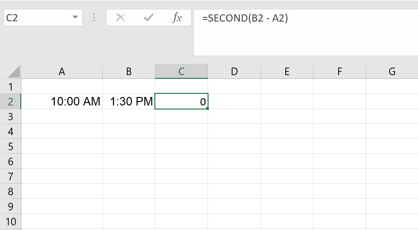

These functions are useful, but they reset after 23 hours, 59 minutes, or 59 seconds. So if the duration is longer than a full day, they won’t reflect the total time elapsed. In those cases, it’s better to multiply the difference or use custom formats, which we’ll cover later.

Add time values over 24 hours

If you need to add hours that exceed 24 hours, direct use of TIME() won’t work as expected. Instead, you can perform arithmetic using fractions of a day.

Here is how you add hours over 24.

=A2 + (28/24)  ' Adds 28 hours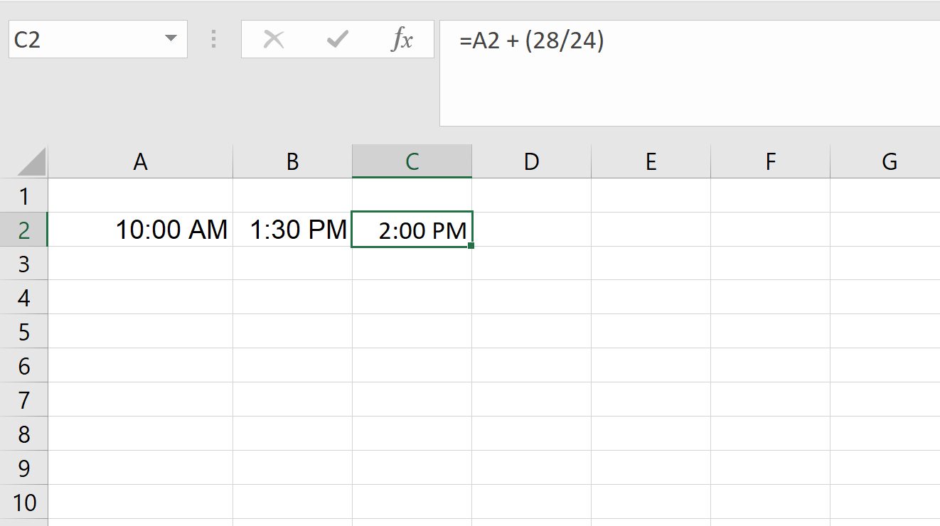

Here is how you add minutes over 60.

=A2 + (90/1440)  ' Adds 90 minutes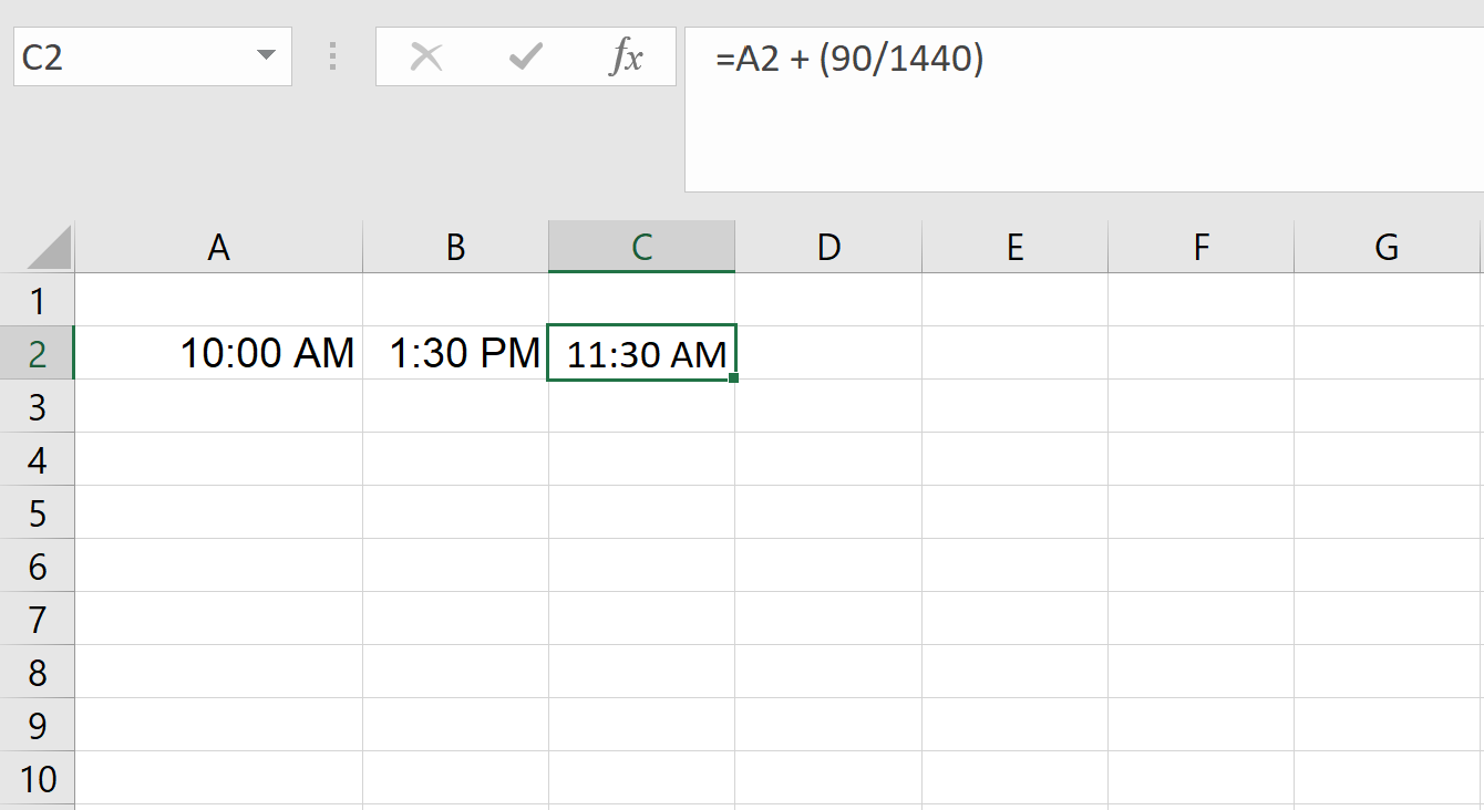

Here is how you add seconds over 60.

=A2 + (3600/86400)  ' Adds 3600 seconds

Excel stores time as a decimal, where 1 day equals 1, so dividing by 24, 1440, or 86400 adjusts the value to represent a portion of a day.

Handle negative time values

By default, if you subtract a larger time from a smaller time (e.g., 10:00 AM - 2:00 PM), Excel will return an error or display a string of ###.

To safely handle negative time values, use the MOD() function. This function effectively prevents negative results by wrapping them around to a valid time.

For example, to subtract 3 hours safely:

=MOD(A2 - TIME(3, 0, 0), 1)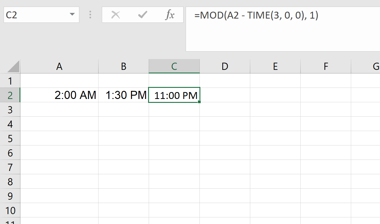

This formula ensures that the result is always a positive time value, preventing unwanted errors or display issues.

How to Format Time Results Correctly

Time calculations in Excel often produce confusing decimal values or unexpected results, especially when dealing with durations over 24 hours or negative time values. Proper formatting can transform raw outputs into readable, user-friendly formats that are easier to interpret and present.

Using basic time formatting

If you want to display a time difference like “3:30” instead of a decimal, use the TEXT() function.

=TEXT(B2 - A2, "h:mm")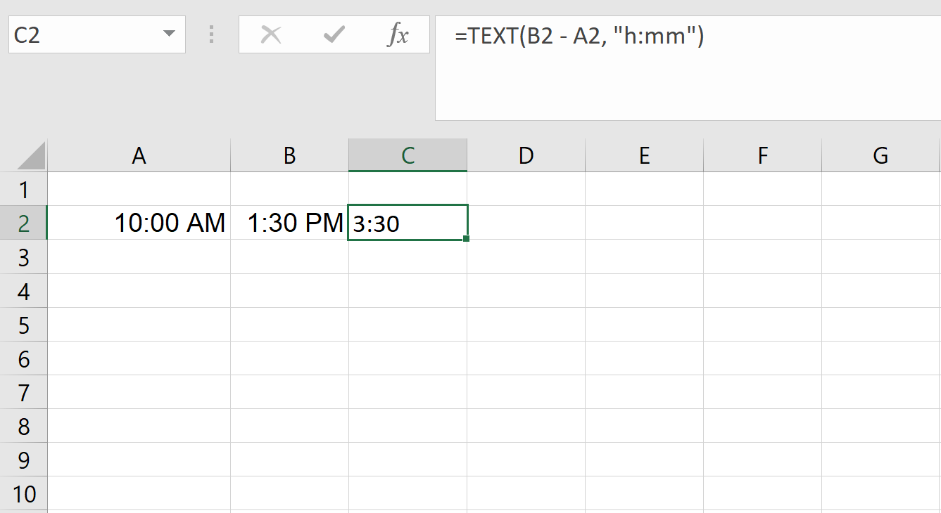

This formats the result as hours and minutes. Just keep in mind that the output is text which looks good but you won’t be able to use it in further math calculations unless you convert it back.

Applying custom time formats

Excel’s built-in time formats handle standard time values effectively, but custom formats provide greater flexibility for displaying durations, extended hours, or specific time components.

To apply a custom time format, follow these steps:

1. Select the cell(s) containing the time values.
2. Right-click and choose Format Cells.
3. In the Number tab, select Custom.
4. Enter the desired format code.

Here are some common custom time formats:

• [h]:mm: Displays total hours and minutes, even beyond 24 hours. Example: 36:45 (36 hours and 45 minutes)

• d "days" h:mm:ss: Displays days, hours, minutes, and seconds. Example: 1 days 12:30:00

• h:mm AM/PM: Displays time with AM/PM notation. Example: 10:30 PM

• mm:ss: Displays only minutes and seconds. Here’s an example: 45:15

Custom formats allow you to present time data in ways that are more intuitive for specific use cases, like timesheets or work logs.

Displaying friendly time differences

If you want to display a time difference as a human-readable string, such as “2 days, 4 hours, and 15 minutes,” you can combine multiple functions in a single formula.

Here’s a practical example:

=INT(B2 - A2) & " days, " & HOUR(B2 - A2) & " hours, " & MINUTE(B2 - A2) & " minutes"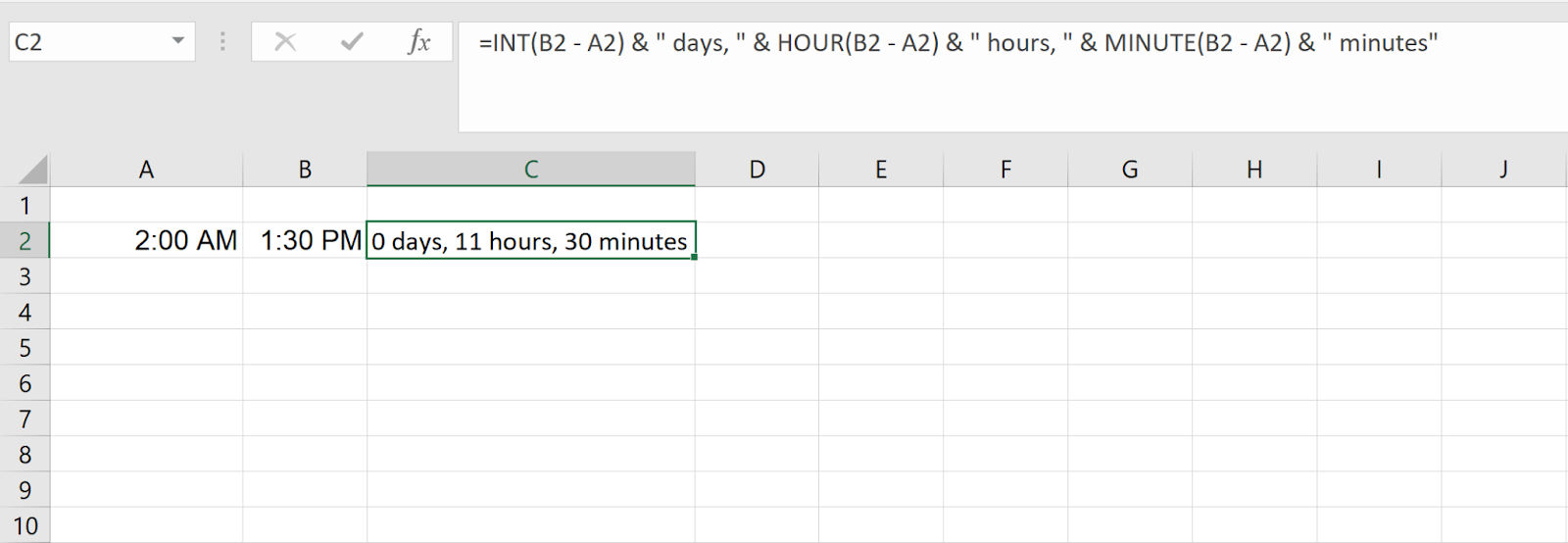

In this formula, the INT() function extracts the number of full days, while HOUR() and MINUTE() pull the remaining hours and minutes.

To prevent zero values from appearing in the output, you can nest these calculations within IF() statements. For instance:

=IF(INT(B2 - A2) > 0, INT(B2 - A2) & " days, ", "") &
 IF(HOUR(B2 - A2) > 0, HOUR(B2 - A2) & " hours, ", "") &
 MINUTE(B2 - A2) & " minutes"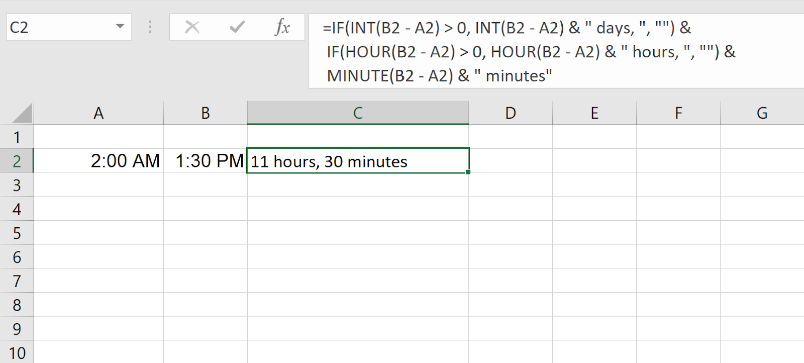

This formula only displays relevant units, making the output cleaner and more readable.

Key Excel Time Functions to Know

As you have seen so far, Excel includes a powerful set of time functions. In the interest of having a more complete accounting, here’s a quick rundown of the most important Excel time functions.

Using the TIME() function to create time values

TIME() constructs a valid time value from three components: hours, minutes, and seconds. This function is ideal when you need to build a time value programmatically.

Here’s a good example:

=TIME(14, 30, 0)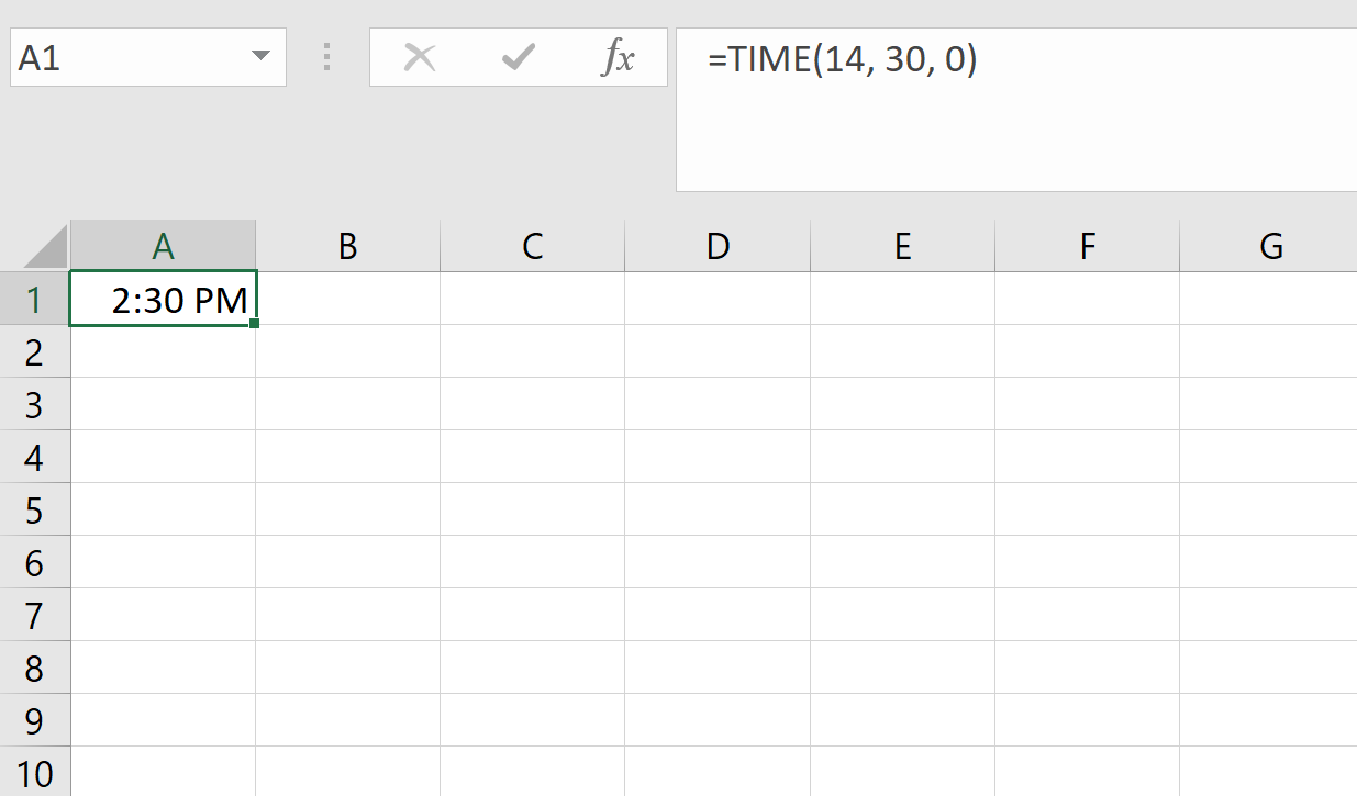  

The above will return 2:30 PM which is a result of this syntax.

=TIME(hour, minute, second)

Converting text to time with TIMEVALUE()

If you have a time written as a text string (e.g., "2:45 PM"), use TIMEVALUE() to convert it to a proper Excel time value that can be used in calculations.

=TIMEVALUE("2:45 PM")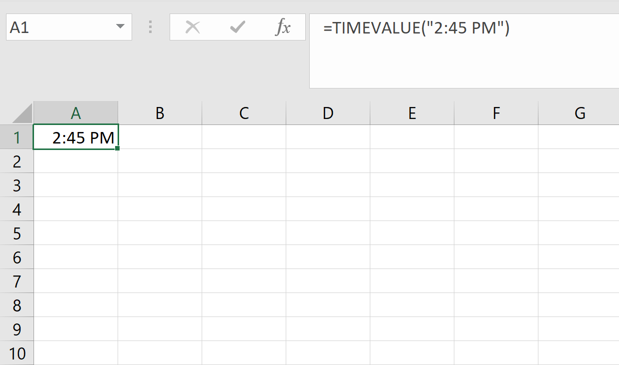

For example, this will return 0.614583 which is a fraction of a day:

=TIMEVALUE("14:45")

Getting the current date and time with NOW()

NOW() returns the current date and time as a single value. It updates automatically whenever the worksheet recalculates.

=NOW()

Here’s a good example. If the current time is 3:15 PM, NOW() might return 44710.63542, where 44710 is the date and .63542 represents the time.

Retrieving the current date with TODAY()

If you only need the current date without time, use TODAY(). This function is particularly useful for calculating deadlines or aging data.

=TODAY()

Extracting time components with HOUR(), MINUTE(), and SECOND()

These functions let you isolate specific parts of a time value, making them useful for reporting and conditional logic.

HOUR() returns the hour portion of a time value (0-23).

=HOUR(A2)

MINUTE() returns the minute portion (0-59).

=MINUTE(A2)

SECOND() returns the seconds portion (0-59).

=SECOND(A2)

Formatting time values with TEXT()

TEXT() converts a time value to a specific format, making it ideal for displaying durations or creating custom time strings. Syntax:

=TEXT(A2, "h:mm:ss AM/PM")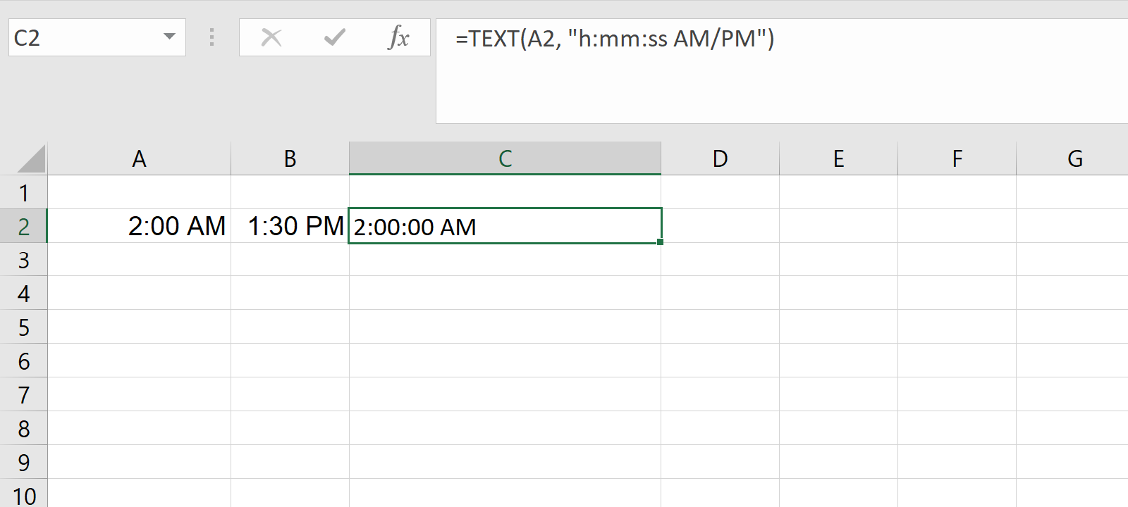

Handling negative time values with TEXT()

When subtracting time values, MOD() ensures that the result is always positive, preventing errors caused by negative time values.

=MOD(A2 - B2, 1)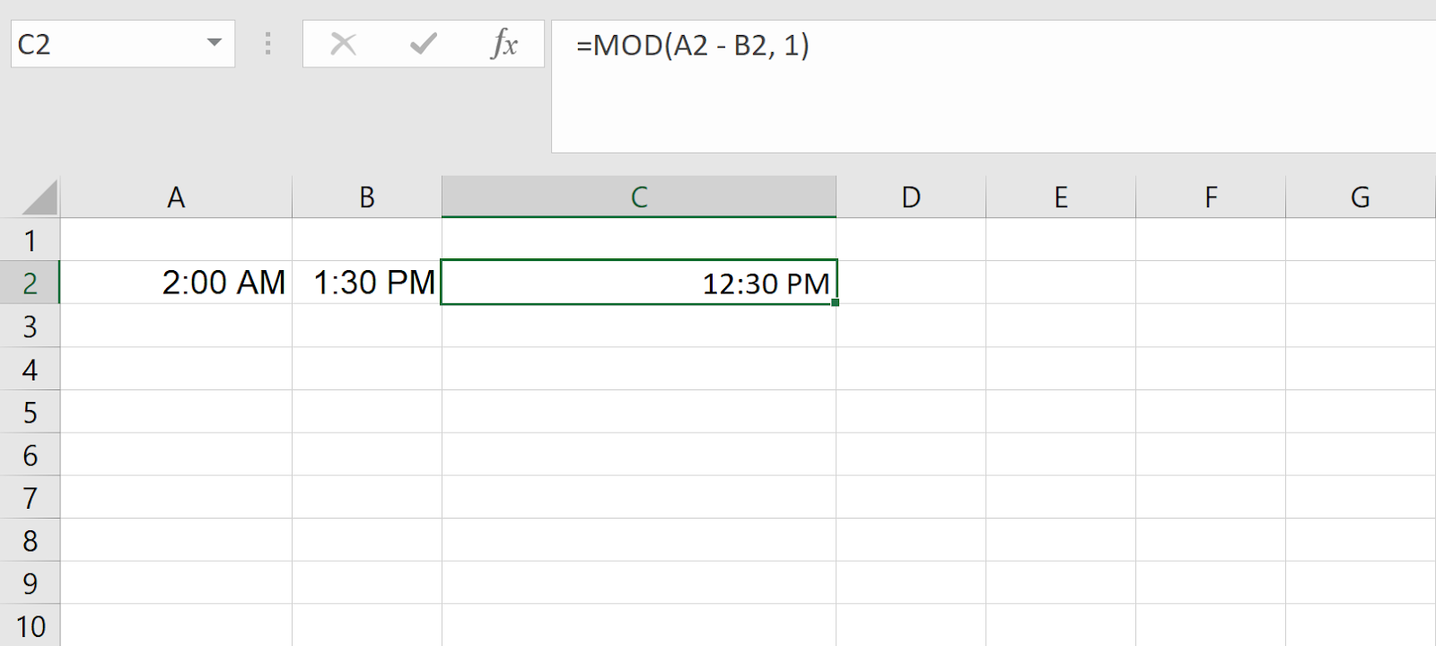

Creating date values with DATE()

DATE() allows you to create a date from separate components: year, month, and day. This is useful for combining dates and times into a single value.

=DATE(year, month, day)

Here’s a good example:

=DATE(2023, 12, 31) + TIME(14, 30, 0)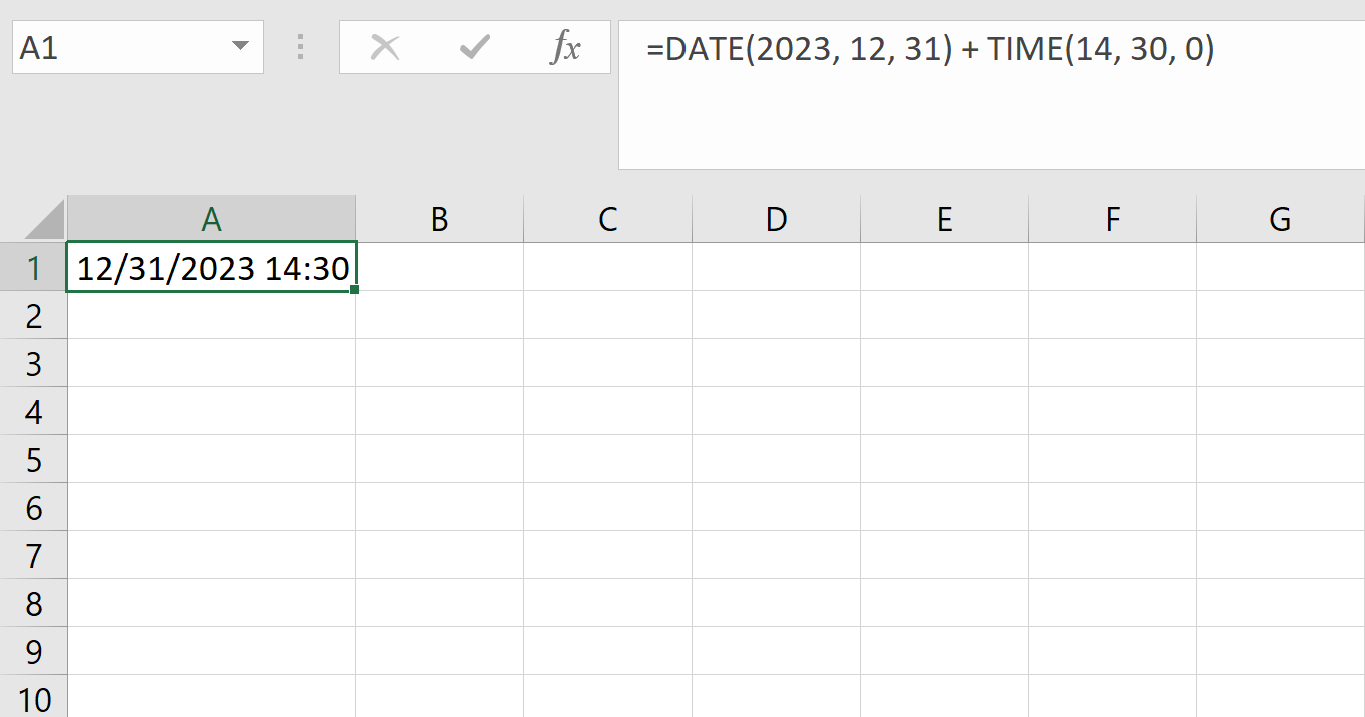

Which returns 12/31/2023 2:30 PM.

Creating working days with NETWORKDAYS()

NETWORKDAYS() calculates the number of workdays between two dates, excluding weekends and optionally specified holidays. This function is ideal for calculating project durations or payroll periods.

=NETWORKDAYS(start_date, end_date, [holidays])

For example:

=NETWORKDAYS(A2, B2, C2:C5)

If A2 contains 12/1/2023 and B2 contains 12/31/2023, the result will be the number of workdays in December, excluding holidays listed in the range C2:C5.

Creating workdays and weekends with WORKDAY.INTL()

WORKDAY.INTL() is an advanced version of WORKDAY() that allows you to customize which days are considered weekends.

=WORKDAY.INTL(start_date, days, [weekend], [holidays])

For example:

=WORKDAY.INTL(A2, 10, "0110000")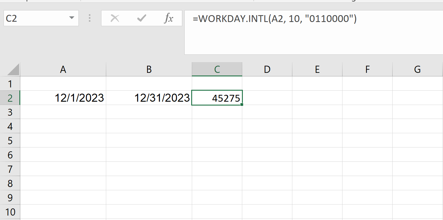

Here, 0110000 specifies that Tuesday (0) and Wednesday (1) are weekends. The formula calculates the date 10 working days after A2, excluding Tuesday and Wednesday.

Conclusion

Handling time in Excel can feel complicated, but with the right functions, it becomes much more manageable.

If you’re looking to strengthen your Excel skills further, check out our Introduction to Excel for foundational skills or the Data Analysis in Excel course to practice working with real-world data.

For more advanced applications, the Excel Fundamentals skill track offers guided projects and exercises to help you master time calculations and beyond.