Excel Compound Interest Formula: A Comprehensive Guide

Understanding compound interest is crucial for financial analysis, as it plays a significant role in personal finance, investment strategies, and business decision-making. Excel helps to simplify these calculations, making it easier to forecast future savings, assess investment returns, and plan loan repayments.

This guide will walk you through different methods for calculating compound interest in Excel, from basic formulas to advanced techniques. Our Financial Modeling in Excel course further builds on the techniques and strategies discussed in this tutorial. Mastering these concepts can significantly improve your financial analysis skills.

What Is Compound Interest?

Compound interest represents the exponential growth of money over time. Unlike simple interest, which grows linearly, compound interest accelerates as the interest earned in each period becomes part of the principal for the next period.

The power of compound interest becomes evident when visualizing long-term investments. Suppose a slight difference in interest rates (like 6% versus 8%) can result in dramatically different outcomes over decades, potentially meaning the difference between a comfortable retirement and financial struggle.

The Compound Interest Formula

Compound interest is calculated using the formula:

Compound interest formula. Image by Author.

Where:

• A = Final amount after interest
• P = Principal (initial investment)
• r = Annual interest rate (in decimal form)
• n = Number of times interest is compounded per year
• t = Number of years

Now that we’ve understood the concept and the mathematical formula, let’s implement it in Excel.

How to Calculate Compound Interest in Excel

To implement this formula in Excel, set up a basic spreadsheet structure with clearly labeled cells for each variable.

First, organize your spreadsheet with the following labels:

• Cell A1: “Principal”
• Cell A2: “Annual Interest Rate”
• Cell A3: “Compounding Periods per Year”
• Cell A4: “Time (years)”
• Cell A5: “Final Amount”

Next, enter your values in column B:

• Cell B1: Enter your principal amount (e.g., 1000)

• Cell B2: Enter your interest rate as a decimal (e.g., 0.05 for 5%)

• Cell B3: Enter the number of compounding periods per year (e.g., 12 for monthly)

• Cell B4: Enter the time in years (e.g., 5)

After setting up the data, your Excel sheet should look like:

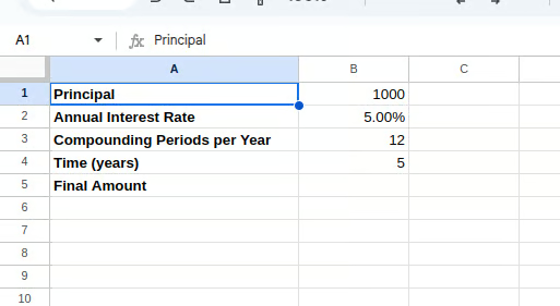
Setting up the Excel table. Image by Author.

Finally, in cell B5, enter the compound interest formula:

=B1*(1+B2/B3)^(B3*B4)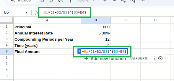

Compound interest formula in Excel. Image by Author.

This formula directly applies the mathematical equation above, calculating the final amount after compound interest.

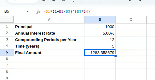
Calculating compound interest. Image by Author.

Using the FV() function

While the manual formula works well, Excel provides built-in financial functions that simplify compound interest calculations. The FV() function (Future Value) is particularly useful for calculating compound interest when making regular payments or investments.

The syntax for the FV() function is:

=FV(rate, nper, pmt, [pv], [type])

Where:

• rate = Interest rate per period

• nper = Total number of payment periods

• pmt = Payment made each period (enter 0 if none)

• pv = Present value (initial principal), should be entered as a negative number

• type = When payments are due (0 for end of period, 1 for beginning)

Let’s modify our spreadsheet to use the FV() function:

• Cell A6: “Using FV() Function”

Type the following in cell B6:

=FV(B2/B3, B3*B4, 0, -B1)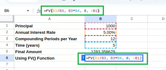

Calculating compound interest using FV(). Image by Author.

Note that we divide the annual interest rate by the number of compounding periods to get the rate per period, and we enter the principal as a negative number as required by the function.

You should be able to see the calculated compound interest as below:

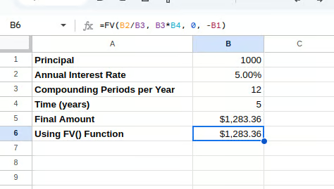
Compound interest using FV(). Image by Author.

Using the PMT() function

The PMT() function calculates the payment for a loan based on constant payments and a constant interest rate. While it's primarily designed for loan payments, it can be adapted for compound interest scenarios where you want to determine regular contribution amounts to reach a target sum.

The syntax for the PMT() function is:

=PMT(rate, nper, pv, [fv], [type])

Where:

• rate = Interest rate per period

• nper = Total number of payment periods

• pv = Present value (initial principal)

• fv = Future value (the target amount you want to reach)

• type = When payments are due (0 for end of period, 1 for beginning)

Let’s add this to our spreadsheet:

• Cell A7: “Target Amount”

• Cell B7: Enter your target amount (e.g., 5000)

• Cell A8: “Required Monthly Payment”

Type the following in cell B8:

=PMT(B2/12, B4*12, -B1, B7)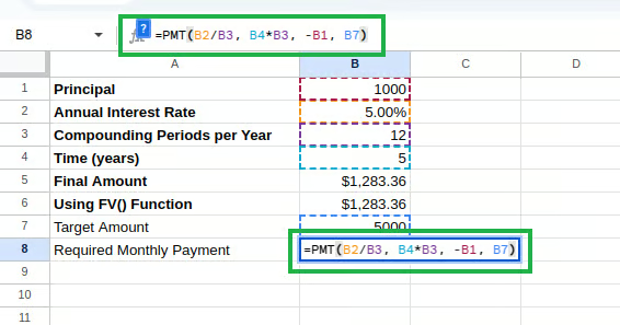

Calculating compound interest using PMT(). Image by Author.

This formula calculates how much you need to contribute monthly to reach your target amount, given your initial principal and interest rate.

The calculated monthly payment can be seen as below:

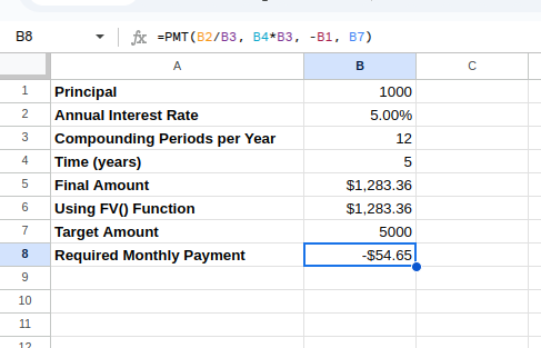
Compound interest using PMT(). Image by Author.

The PMT() function in Excel returns a negative value by default because it’s designed from a cash flow perspective:

• Negative values represent money that you pay out (cash outflow)
• Positive values represent money that you receive (cash inflow)

Excel Compound Interest in Action

The compound interest formula in Excel has numerous real-world applications across personal finance and business contexts. Let’s explore some of these practical scenarios.

Savings and investments

One of the most common applications of compound interest calculations is projecting the growth of savings or investment accounts. Understanding how money grows over time can help us make informed decisions.

Let’s create a retirement savings projection model in a new section of our spreadsheet. After entering “Retirement Savings Projection” on cell cell D1, you can setup your parameters in cells D2 through D6:

• Cell D2: “Initial Investment” with E2: 10000

• Cell D3: “Monthly Contribution” with E3: 500

• Cell D4: “Annual Interest Rate” with E4: 0.07

• Cell D5: “Time Horizon (years)” with E5: 30

• Cell D6: “Compounding Frequency” with E6: “Monthly”

After entering “Projected Future Value” in cell D7, type the following equation in E7:

=FV(E4/12, E5*12, -E3, -E2)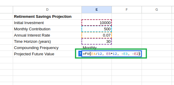

Calculating projected future value. Image by Author.

This formula projects your retirement savings, accounting for both your initial investment and regular contributions. You can see the future value as below:

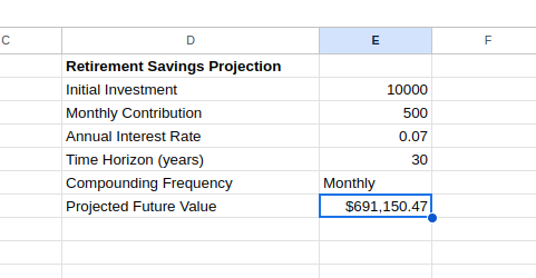
Projected future value using FV(). Image by Author.

We can enhance this model by creating a year-by-year projection table:

• In cell D9, enter “Year-by-Year Projection”

• In cell D10, enter “Year” and in cell E10, enter “Balance”

• In cell D11, enter 0 (starting year)

• In cell E11, enter your initial investment: =E2

• In cell D12, enter 1

• In cell E12, calculate the balance after year 1:

=FV($E$4/12, 1*12, -$E$3, -E11)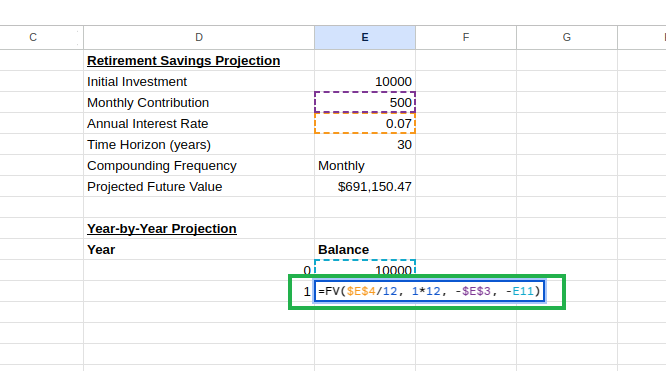

Creating a year-by-year projection table. Image by Author.

• Select cells D11 and D12, then click and drag the fill handle (small square at the bottom-right corner) down to row 41 to create years 0 through 30
• Select cell E12, then click and drag the fill handle down to row 41

Excel will automatically adjust the cell references in each row, creating a sequence of calculations where each year builds upon the previous year’s balance.

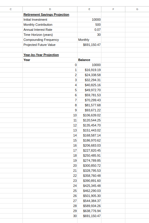
Year-by-year projection table. Image by Author.

This chart can help you understand how your savings grow over time and can motivate consistent investing by illustrating the accelerating growth pattern typical of compound interest.

Loan calculations

Compound interest also applies to loans, where interest compounds on the remaining balance. Excel’s functions can help you understand various aspects of loans, from monthly payments to total interest paid.

To create a loan amortization schedule, set up your loan parameters as shown below:

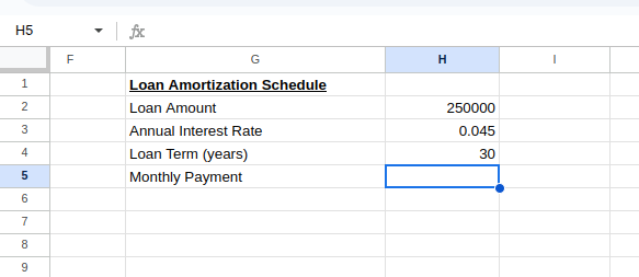Calculating the loan's monthly payment. Image by Author.

On cell H3, type the following to calculate the monthly payment:

=PMT(H3/12, H4*12, H2)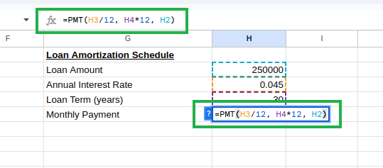

Calculating loan monthly payment using PMT(). Image by Author.

You’d see the monthly payment as:

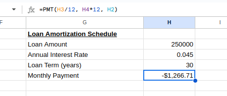
Loan monthly payment. Image by Author.

Next, set up the amortization schedule table with a header as below:

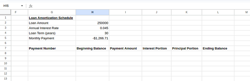Creating amortization schedule table. Image by Author.

Enter the initial values for the first payment (row 8):

• Cell G8: 1 (first payment)

• Cell H8: =H2 (initial loan amount)

• Cell I8: =ABS(H5) (payment amount, using ABS() to convert negative PMT() result to positive)

• Cell J8: =H8*($H$3/12) (interest portion: beginning balance × monthly rate)

• Cell K8: =I8-J8 (principal portion: payment amount − interest portion)

• Cell L8: =H8-K8 (ending balance: beginning balance − principal portion)

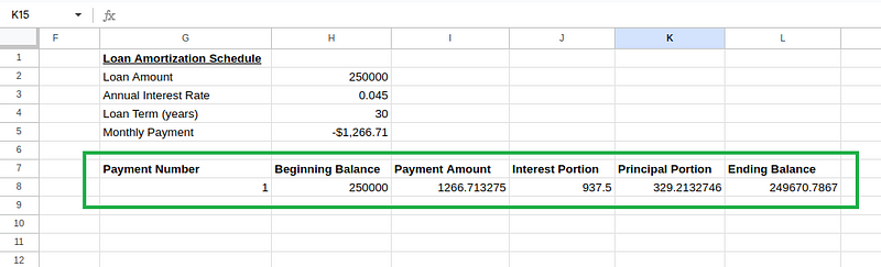Amortization schedule table calculations. Image by Author.

For the second payment (row 9), create the following formulas:

• Cell G9: 2 (second payment)

• Cell H9: =L8 (beginning balance equals previous payment’s ending balance)

• Cell I9: =I8 (payment amount stays the same)

• Cell J9: =H9*($H$3/12) (interest portion based on new beginning balance)

• Cell K9: =I9-J9 (principal portion)

• Cell L9: =H9-K9 (ending balance)

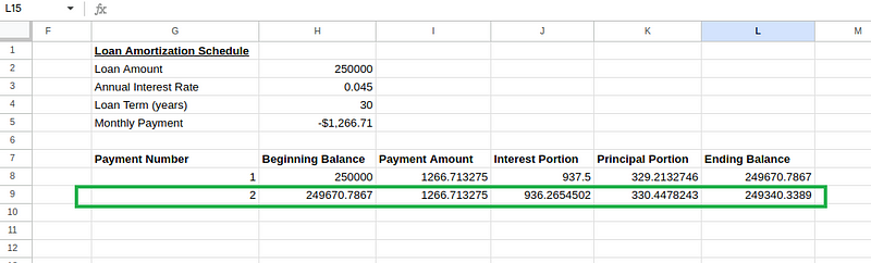Amortization schedule table calculations. Image by Author.

Then select cells H9 to L9 and drag down to row 367 (for all 360 payments).

In cell H6, we can calculate the total interest paid: 

=SUM(J8:J367)

The final schedule should look like:

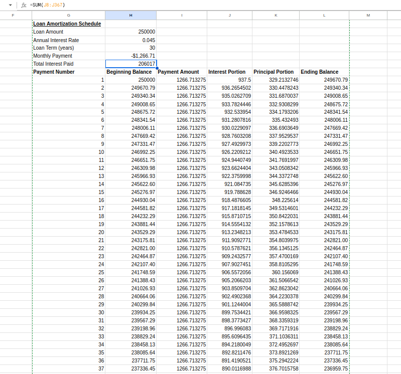Amortization schedule table. Image by Author.

This amortization schedule reveals how each payment affects your loan balance and the substantial amount of interest paid over the loan’s lifetime. Early payments primarily cover interest, while later payments mainly reduce principal — an important insight for understanding mortgage loans.

Advanced Compound Interest Techniques

Let’s explore scenarios in which some advanced techniques are used, such as handling irregular compounding periods and varying interest rates.

Variable interest rates

Real-world scenarios often involve variable interest rates, such as adjustable-rate mortgages or market-linked investments. Excel can handle these complex scenarios with some additional setup.

We can create a model with different interest rates for different time periods. Let’s set up a variable interest rate table assuming that interest rates are to increase by 0.5% every 5 years:

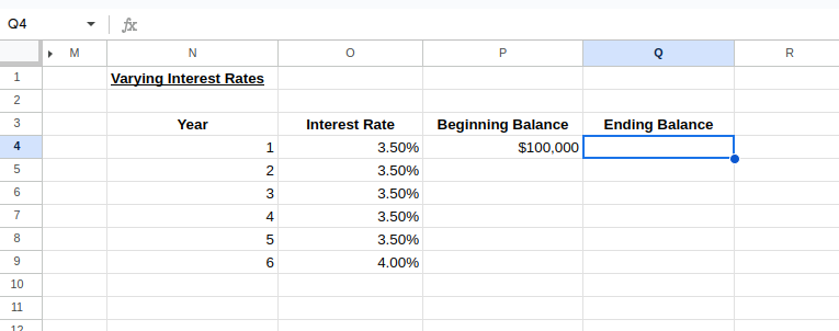Setting up a table for varying interest rates. Image by Author.

To calculate the ending balance of Year 1 and the beginning balance of Year 2, type the following:

• Cell Q4: =P4*(1+O4)

• Cell P5: =Q4

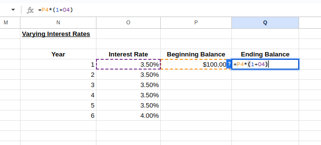Varying interest rates calculations. Image by Author.

We can now select the rows of Years 1–2 and drag down to extend the table to our desired number of years, modifying interest rates as needed, as shown in the image below:

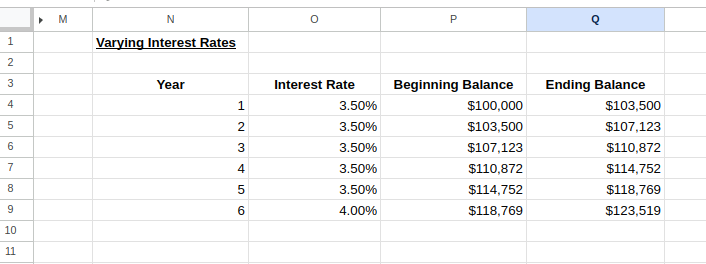Varying interest rate calculator. Image by Author.

This model lets you visualize how changing interest rates affect your investment or loan over time. 

Compounding frequency

Real-world financial products often use non-standard compounding periods. Some investments compound quarterly, others monthly, and some even daily. These differences in compounding frequency can significantly impact your returns over time.

To accommodate these variations in Excel, you can adjust the compound interest formula accordingly. Suppose calculating a $10,000 investment at 6% annual interest with daily compounding for 5 years would use this formula:

=10000*(1+0.06/365)^(365*5)

A sample irregular compounding calculator will look like:

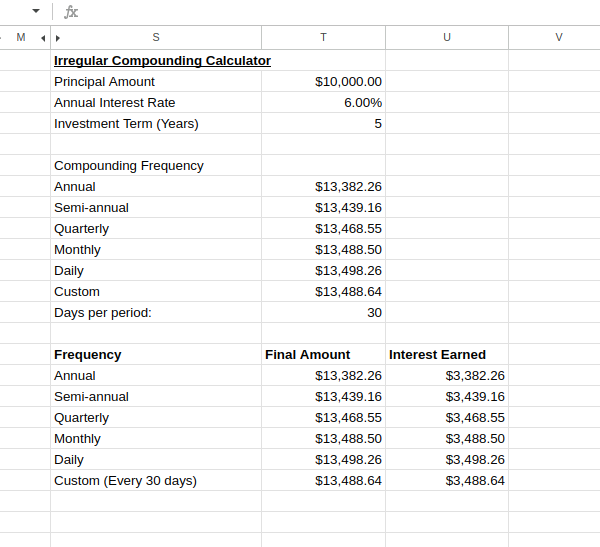Irregular compounding calculator. Image by Author.

This comparison clearly demonstrates how compounding frequency affects your investment returns.

As you can see, more frequent compounding yields higher returns, though the incremental benefit diminishes as frequency increases. This insight is particularly valuable when evaluating financial products that advertise different compounding methods.

Conclusion

Throughout this guide, we’ve explored various practical applications of Excel’s compound interest formulas. From understanding the fundamental mathematical formula to implementing Excel’s financial functions like FV() and PMT(), we now have the essential tools to perform meaningful financial calculations.

To deepen your Excel skills beyond this tutorial, consider enrolling in our Financial Modeling in Excel course. This course builds upon the fundamental concepts discussed in the tutorial with advanced financial modeling techniques.