Remove Blank Rows in Excel: 4 Easy Methods

Blank rows in Excel often appear when you export data from other systems, when you accidentally leave gaps, or when you combine different sheets. These gaps can disrupt important tasks such as data sorting, filtering, and analysis. They slow you down, and if you're not careful, they can lead to mistakes.

In this article, I'll show you four different ways to remove these blank rows.

Quick Answer: Remove a Blank Row

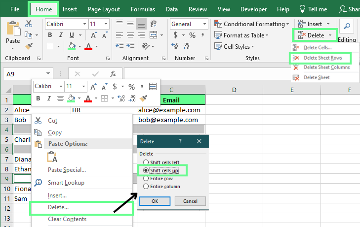
To delete a blank row in Excel:

1. Select the row you want to delete. To select multiple rows, hold Ctrl while clicking each one.

2. Right-click and choose Delete.

3. In the pop-up window, select Shift cells up.

Methods to Delete Blank Rows in Excel

Here’s a step-by-step breakdown of different methods you can use to delete blank rows with clear examples to guide you quickly.

Method 1: Delete only completely blank rows using COUNTA()

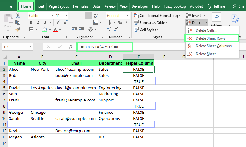
The COUNTA() function counts the number of non-empty cells in a range. We can use it to spot completely blank rows. This is quite helpful when we want to avoid removing rows with partial data.

Here’s how you can use this to delete a row:

1. Create a helper column next to the dataset. In the first cell, enter =COUNTA(A2:C2)=0. 

2. Drag the formula down to copy it. This will display True if the entire row is blank and False if it contains any non-blank values. 

3. Now click on the True cells, go to the Home tab, and click Delete Sheet Rows to delete the whole row at once.

Method 2: Use FILTER() for formula-based data cleanup

The FILTER() function doesn’t delete rows. It returns a new, blank-free version of your data in a separate range. You can use it to preserve your original data while working with a cleaned-up view. But note that FILTER() is only available in Excel 365 and Excel 2021.

Here I have a dataset with blank rows, and to clean the blank rows, I use the following formula (adjust ranges according to your data):

=FILTER(A2:A10, NOT(ISBLANK(A2:A10)))

In this formula:

• FILTER() returns data from a range that meets a condition.

• A2:A10 is the range being filtered.

• ISBLANK(A2:A10) checks for blank cells.

• NOT(...) reverses the result, so only non-blank cells from Column A are returned and skip any blanks.

This method only works with one column at a time. So if you’re working with multiple columns, you’ll need to adjust the formula by selecting the new column and dragging it horizontally.

Method 3: Use sort to push blank rows to the bottom

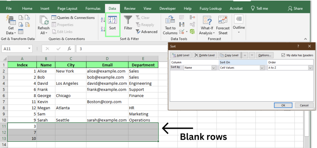
Sorting in Excel reorders data based on the values in one or more columns. For example, sorting a name column from A to Z rearranges the entire table so names are in alphabetical order while keeping each row's data intact.

When you sort a column, Excel moves all blank rows to the bottom of the sheet. That makes it easy to scroll down and delete them in one go.

Here’s how to do it:

1. Select your data.
2. Go to the Data tab and click Sort.
3. In the Sort dialog box, choose any column (except one with just numbers), leave the settings as-is, and click OK.
4. Excel will sort your data in ascending order, pushing blank rows to the bottom.
5. Select those empty rows, right-click, and Delete them.

To preserve your original order, add an index column before sorting. After deleting the blanks, sort again using the index to restore the original layout, then remove the index column.

Method 4: Use VBA to remove blank rows automatically

VBA (Visual Basic for Applications) automates many Excel tasks, including removing multiple blank rows simultaneously. Here’s a simple way to do it:

• Press Alt + F11 to open the Visual Basic Editor.

• Click Insert > Module to create a new module.

• Paste the following code into the module:

Sub DeleteBlankRows()
    Dim rng As Range
    Dim row As Range

    On Error Resume Next
    Set rng = ActiveSheet.UsedRange

    For Each row In rng.Rows
        If Application.WorksheetFunction.CountA(row) = 0 Then
            row.Delete
        End If
    Next row
End Sub

Close the editor and press Alt + F8 to run the macro called DeleteBlankRows. This will delete only rows that contain all empty cells and won’t affect rows that have only a few blank cells. 

Comparing the Different Methods

Here's a quick table to help you see how all the methods we talked about stack up against each other. 

Before you start deleting, remember that some blank rows might be intentional, like when they’re used to separate sections and make your data easier to read. In those cases, it may be better to hide the rows or use conditional formatting instead. Always choose the method that best fits your data and goals.

If you want to improve your overall Excel skills, check out courses like Data Analysis in Excel or Data Visualization in Excel. They’re great for building skills you’ll actually use.