Speculative Decoding: A Guide With Implementation Examples

LLMs are so powerful, but they can often be a bit slow, and this is not ideal in scenarios where we need speed. Speculative decoding is a technique designed to speed LLMs by generating responses faster without compromising quality.

In essence, it’s a way to “guess ahead” in the process of text generation, making predictions about the words that might come next while still allowing for the accuracy and depth we expect from LLMs.

In this blog, I’ll explain what speculative decoding is, how it works, and how to implement it with Gemma 2 models.

What Is Speculative Decoding?

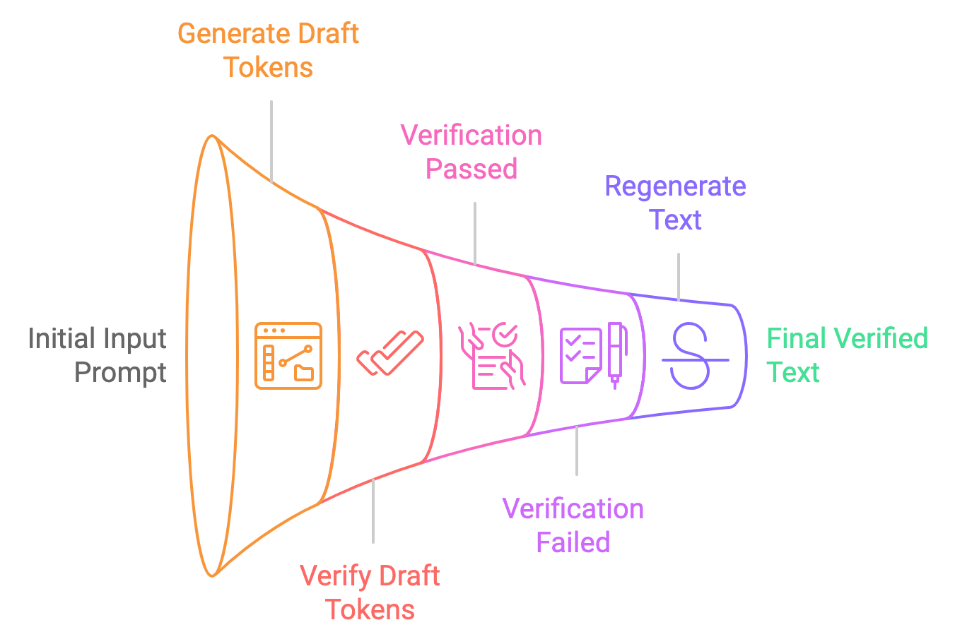
Speculative decoding accelerates LLMs by incorporating a smaller, faster model that generates preliminary predictions. This smaller model, often called the “draft” model, generates a batch of tokens that the main, more powerful LLM can either confirm or refine. The draft model acts as a first pass, producing multiple tokens that speed up the generation process.

Instead of the main LLM generating tokens sequentially, the draft model provides a set of likely candidates, and the main model evaluates them in parallel. This method reduces the computational load on the main LLM by offloading initial predictions, allowing it to focus only on corrections or validations.

Think of it like a writer with an editor. The main LLM is the writer, capable of producing high-quality text but at a slower pace. A smaller, faster "draft" model acts as the editor, quickly generating potential continuations of the text. The main LLM then evaluates these suggestions, incorporating the accurate ones and discarding the rest. This allows the LLM to process multiple tokens concurrently, speeding up text generation.

Let's break down the process of speculative decoding into simple steps:

1. ​Draft generation: The smaller model (e.g., Gemma2-2B-it) generates multiple token suggestions based on the input prompt. These tokens are generated speculatively, meaning the model is not certain they are correct but provides them as “draft” tokens.
2. Parallel ​verification: The larger model (e.g., Gemma2-9B-it) verifies these tokens in parallel, checking their probability against the model’s learned distribution. If the tokens are deemed acceptable, they are used in the final output. If not, the larger model corrects them.
3. ​Final output: Once the tokens are verified (or corrected), they are passed on to the user as the final output. This entire process happens much faster than traditional one-token-at-a-time decoding.

Traditional Decoding vs. Speculative Decoding

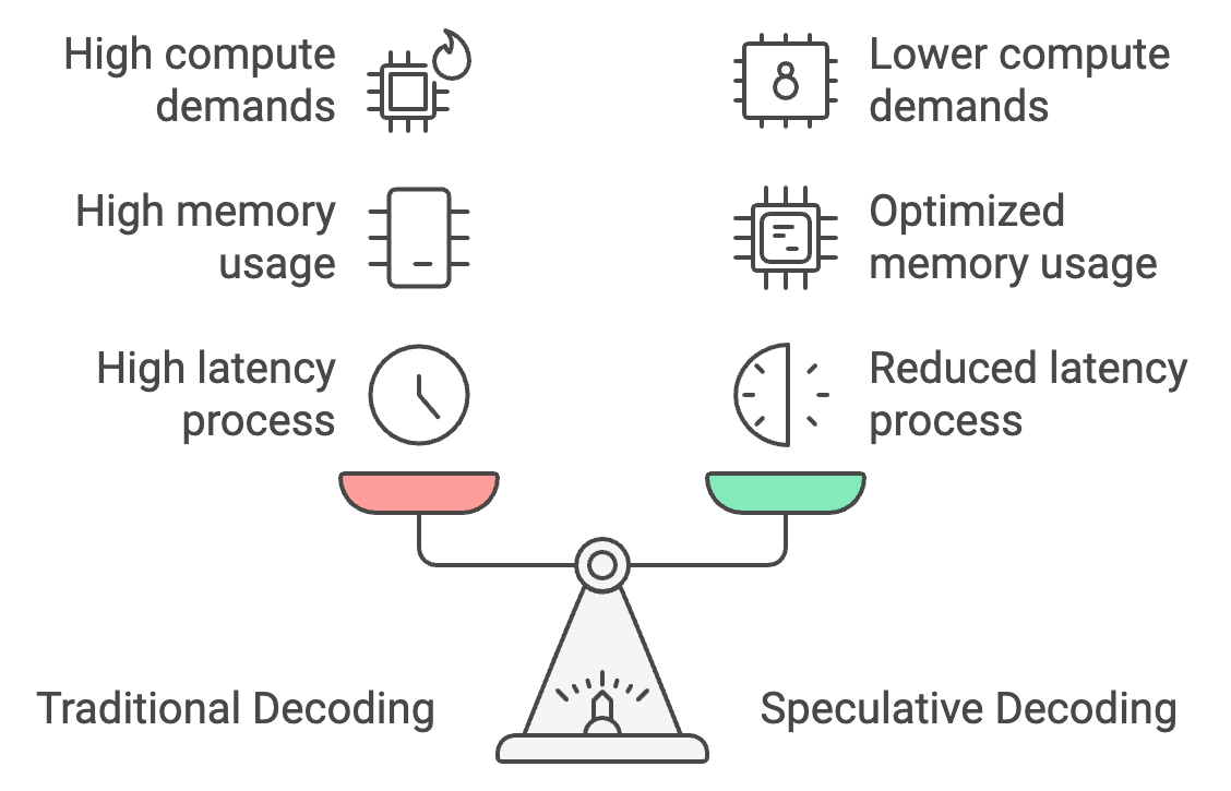
Traditional decoding processes tokens one at a time, leading to high latency, but speculative decoding allows a smaller model to generate tokens in bulk, with the larger model verifying them. This can reduce response time by 30-40%, cutting latency from 25-30 seconds to as little as 15-18 seconds.

Additionally, speculative decoding optimizes memory usage by shifting most of the token generation to the smaller model, reducing memory requirements from 26 GB to around 14 GB and making on-device inference more accessible.

Finally, it lowers compute demands by 50%, as the larger model only verifies rather than generates tokens, enabling smoother performance on mobile devices with limited power and preventing overheating.

Hands-On Example: Speculative Decoding With Gemma2 Models

To implement a hands-on example of speculative decoding using the Gemma2 models. We’ll explore how speculative decoding compares with standard inference in terms of both latency and performance.

Step 1: Model and Tokenizer setup

To get started, import the dependencies and set the seed.

Next, check if GPU is available on the machine you are operating on. This is mainly required for big models such as Gemma 2-9B-it or LLama2-13B.

Finally, we load both small and big model along with their tokenizers. Here, we are using the Gemma2-2b-it (instruct) model for the draft model and the Gemma2-9b-it model for verification.

There are a few other models that can be used alternatively as well. For example:

• Gemma 7B (main) & Gemma 2B (draft)
• Mixtral-8x7B (main) & Mistral 7B (draft)
• Pythia 12B (main) & Pythia 70M (draft)
• Llama 2 13B (main) & TinyLlama 1.1B (draft)

import torch
from transformers import AutoTokenizer, AutoModelForCausalLM, set_seed

# Set Seed
set_seed(42)

# Check if GPU is available
device = "cuda" if torch.cuda.is_available() else "cpu"

# Load the smaller Gemma2 model (draft generation)
small_tokenizer = AutoTokenizer.from_pretrained("google/gemma-2-2b-it", device_map="auto")
small_model = AutoModelForCausalLM.from_pretrained("google/gemma-2-2b-it", device_map="auto", torch_dtype=torch.bfloat16)

# Load the larger Gemma2 model (verification)
big_tokenizer = AutoTokenizer.from_pretrained("google/gemma-2-9b-it", device_map="auto")
big_model = AutoModelForCausalLM.from_pretrained("google/gemma-2-9b-it", device_map="auto", torch_dtype=torch.bfloat16)

Step 2: Autoregressive (normal) inference 

First, we perform inference on just the large model (Gemma2-9b-it) and generate output. Start by tokenizing the input prompt and moving the tokens to the correct device (GPU if available). The generate method produces the model's output, generating up to max_new_tokens. The result is then decoded from token IDs back into human-readable text.

def normal_inference(big_model, big_tokenizer, prompt, max_new_tokens=50):
    inputs = big_tokenizer(prompt, return_tensors='pt').to(device)
    outputs = big_model.generate(inputs['input_ids'], max_new_tokens=max_new_tokens)
    return big_tokenizer.decode(outputs[0], skip_special_tokens=True)

Step 3: Speculative decoding 

Next, we try the speculative decoding method, where we take the following steps:

1. Draft generation: The smaller model generates a draft of the text from the given prompt.
2. Verification: The larger model then verifies the draft by computing the log-likelihood for each token in the draft.
3. Log-likelihood calculation: We compute an average log-likelihood to determine how likely the large model considers the small model’s draft to be correct.

def speculative_decoding(small_model, big_model, small_tokenizer, big_tokenizer, prompt, max_new_tokens=50):
    # Step 1: Use the small model to generate the draft
    inputs = small_tokenizer(prompt, return_tensors='pt').to(device)
    small_outputs = small_model.generate(inputs['input_ids'], max_new_tokens=max_new_tokens)
    draft = small_tokenizer.decode(small_outputs[0], skip_special_tokens=True)

    # Step 2: Verify the draft with the big model
    big_inputs = big_tokenizer(draft, return_tensors='pt').to(device)

    # Step 3: Calculate log-likelihood of the draft tokens under the large model
    with torch.no_grad():
        outputs = big_model(big_inputs['input_ids'])
        log_probs = torch.log_softmax(outputs.logits, dim=-1)

    draft_token_ids = big_inputs['input_ids']
    log_likelihood = 0
    for i in range(draft_token_ids.size(1) - 1):
        token_id = draft_token_ids[0, i + 1]
        log_likelihood += log_probs[0, i, token_id].item()

    avg_log_likelihood = log_likelihood / (draft_token_ids.size(1) - 1)

    # Return the draft and its log-likelihood score
    return draft, avg_log_likelihood

Note: Log-likelihood is the logarithm of the probability that a model assigns to a specific sequence of tokens. Here, it reflects how likely or "confident" the model is that the sequence of tokens (the generated text) is valid given the previous tokens.

Step 4: Measuring latency

After implementing both techniques, we can measure their respective latencies. For speculative decoding, we assess performance by examining the log-likelihood value. A log-likelihood value approaching zero, particularly in the negative range, indicates that the generated text is accurate.

def measure_latency(small_model, big_model, small_tokenizer, big_tokenizer, prompt, max_new_tokens=50):
    # Measure latency for normal inference (big model only)
    start_time = time.time()
    normal_output = normal_inference(big_model, big_tokenizer, prompt, max_new_tokens)
    normal_inference_latency = time.time() - start_time
    print(f"Normal Inference Output: {normal_output}")
    print(f"Normal Inference Latency: {normal_inference_latency:.4f} seconds")
    print("\n\n")

    # Measure latency for speculative decoding
    start_time = time.time()
    speculative_output, log_likelihood = speculative_decoding(
        small_model, big_model, small_tokenizer, big_tokenizer, prompt, max_new_tokens
    )
    speculative_decoding_latency = time.time() - start_time
    print(f"Speculative Decoding Output: {speculative_output}")
    print(f"Speculative Decoding Latency: {speculative_decoding_latency:.4f} seconds")
    print(f"Log Likelihood (Verification Score): {log_likelihood:.4f}")

    return normal_inference_latency, speculative_decoding_latency

This returns:

• Log-likelihood (verification score): -0.5242
• Normal inference latency: 17.8899 seconds
• Speculative decoding latency: 10.5291 seconds (about 70% faster)

The lower latency is thanks to less time taken by the smaller model for text generation and less time taken by the larger model for just verifying the generated text.

Testing Speculative Decoding on Five Prompts

Let's compare speculative decoding with autoregressive inference by using five prompts:

# List of 5 prompts
prompts = [
    "The future of artificial intelligence is ",
    "Machine learning is transforming the world by ",
    "Natural language processing enables computers to understand ",
    "Generative models like GPT-3 can create ",
    "AI ethics and fairness are important considerations for "
]

# Inference settings
max_new_tokens = 200

# Initialize accumulators for latency, memory, and tokens per second
total_tokens_per_sec_normal = 0
total_tokens_per_sec_speculative = 0
total_normal_latency = 0
total_speculative_latency = 0

# Perform inference on each prompt and accumulate the results
for prompt in prompts:
    normal_latency, speculative_latency, _, _, tokens_per_sec_normal, tokens_per_sec_speculative = measure_latency_and_memory(
        small_model, big_model, small_tokenizer, big_tokenizer, prompt, max_new_tokens
    )
    total_tokens_per_sec_normal += tokens_per_sec_normal
    total_tokens_per_sec_speculative += tokens_per_sec_speculative
    total_normal_latency += normal_latency
    total_speculative_latency += speculative_latency

# Calculate averages
average_tokens_per_sec_normal = total_tokens_per_sec_normal / len(prompts)
average_tokens_per_sec_speculative = total_tokens_per_sec_speculative / len(prompts)
average_normal_latency = total_normal_latency / len(prompts)
average_speculative_latency = total_speculative_latency / len(prompts)

# Output the averages
print(f"Average Normal Inference Latency: {average_normal_latency:.4f} seconds")
print(f"Average Speculative Decoding Latency: {average_speculative_latency:.4f} seconds")
print(f"Average Normal Inference Tokens per second: {average_tokens_per_sec_normal:.2f} tokens/second")
print(f"Average Speculative Decoding Tokens per second: {average_tokens_per_sec_speculative:.2f} tokens/second")

Average Normal Inference Latency: 25.0876 seconds
Average Speculative Decoding Latency: 15.7802 seconds
Average Normal Inference Tokens per second: 7.97 tokens/second
Average Speculative Decoding Tokens per second: 12.68 tokens/second

This shows that speculative decoding is more efficient, generating more tokens per second than normal inference. This improvement is because the smaller model handles the majority of the text generation, while the larger model's role is limited to verification, reducing the overall computational load in terms of latency and memory. 

With these memory requirements, we can easily deploy speculative decoding techniques on edge devices and gain speed-ups on our on-device applications such as chatbots, language translators, games, and more.

Optimized Speculative Decoding With Quantization  

The above approach is efficient, but there is a trade-off between latency and memory optimization for on-device inference. To address this, let’s apply quantization to both small and big models. You can experiment and try applying quantization to only the large model since the small model already takes the least space.

Quantification is applied to smaller and larger models using the BitsAndBytesConfig configuration from the Hugging Face transformers library. Quantization allows us to significantly reduce memory usage and, in many cases, improve inference speed by converting the model’s weights to a more compact form.

Add the following code snippet to the above code to witness the effects of quantization.

bnb_config = BitsAndBytesConfig(
    load_in_4bit=True,  # Enables 4-bit quantization
    bnb_4bit_quant_type="nf4",  # Specifies the quantization type (nf4)
    bnb_4bit_compute_dtype=torch.bfloat16,  # Uses bfloat16 for computation
    bnb_4bit_use_double_quant=False,  # Disables double quantization to avoid additional overhead
)

# Load the smaller and larger Gemma2 models with quantization applied
small_model = AutoModelForCausalLM.from_pretrained("google/gemma-2-2b-it", device_map="auto", quantization_config=bnb_config)
big_model = AutoModelForCausalLM.from_pretrained("google/gemma-2-9b-it", device_map="auto", quantization_config=bnb_config)

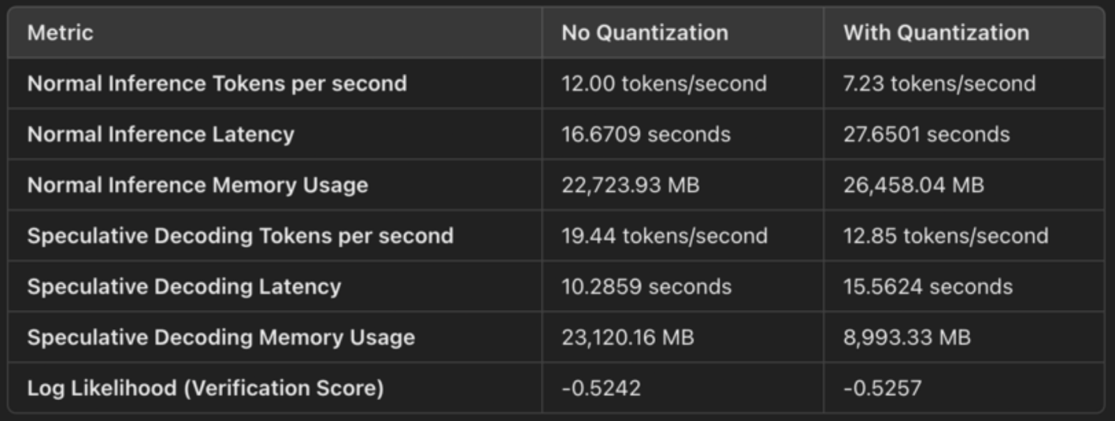
Here is a quick comparison of outputs to showcase the effects of speculative decoding with and without quantization:

4-bit quantization (weight compression)

The configuration specifies load_in_4bit=True, which means the model’s weights are quantized from their original 32-bit or 16-bit floating-point format to 4-bit integers. This reduces the model's memory footprint. Quantization compresses the model’s weights, allowing us to store and operate on them more efficiently. These are the concrete memory savings:

• By reducing the precision from 32-bit or 16-bit floats to 4-bit integers, each weight now takes up 1/4th or 1/8th of the original space, significantly reducing memory usage.
• This is reflected in the memory usage as:
• Normal inference memory usage: 26,458 MB
• Speculative decoding memory usage: 8,993 MB.

bfloat16 for computation (efficient use of Tensor Cores)

The configuration bnb_4bit_compute_dtype=torch.bfloat16 specifies that the computation is performed in bfloat16 (BF16), a more efficient floating-point format. BF16 has a wider dynamic range than FP16 but takes up half the memory compared to FP32, making it a good balance between precision and performance.

Using BF16, especially on NVIDIA GPUs (like A100), uses Tensor Cores, which are optimized for BF16 operations. This results in faster matrix multiplications and other computations during inference.

For speculative decoding, we see improved latency:

• Normal inference latency: 27.65 seconds
• Speculative decoding latency: 15.56 seconds

The smaller memory footprint means faster memory access and more efficient use of GPU resources, leading to faster generation.

NF4 quantization type (optimized precision)

The bnb_4bit_quant_type="nf4" option specifies Norm-Four Quantization (NF4), which is optimized for neural networks. NF4 quantization helps retain the precision of important parts of the model, even though the weights are represented in 4 bits. This minimizes the degradation in model performance compared to simple 4-bit quantization.

NF4 helps achieve a balance between the compactness of 4-bit quantization and the accuracy of the model's predictions, ensuring that performance remains close to the original while drastically reducing memory usage.

Double quantization disabled 

Double quantization (bnb_4bit_use_double_quant=False) introduces an additional layer of quantization on top of the 4-bit weights, which can further reduce memory usage but also add computation overhead. In this case, double quantization is disabled to avoid slowing down the inference.

Applications of Speculative Decoding

The potential applications of speculative decoding are vast and exciting. Here are a few examples:

• Chatbots and virtual assistants: To make those conversations with AI feel more natural and fluid with faster response times.
• Real-time translation: Speculative decoding reduces latency in real-time translation.
• Content generation: Speculative decoding speeds up content creation.
• Gaming and interactive applications: To improve the responsiveness of AI-powered characters or game elements for a more immersive experience, speculative decoding can help us attain almost real-time responses.

Challenges of Speculative Decoding

While speculative decoding holds immense promise, it's not without its challenges:

• Memory overhead: Maintaining multiple model states (for both the draft and main LLM) can increase memory usage, especially when larger models are used for verification.
• Tuning the draft model: Choosing the right draft model and tuning its parameters is crucial to strike the right balance between speed and accuracy, as an overly simplistic model may lead to frequent verification failures.
• Implementation complexity: Implementing speculative decoding is more complex than traditional methods, requiring careful synchronization between the small draft model and the larger verification model, as well as efficient error handling.
• Compatibility with decoding strategies: Speculative decoding currently supports only greedy search and sampling, limiting its use to more sophisticated decoding strategies such as beam search or diverse sampling.
• Verification overhead: If the smaller draft model generates tokens that frequently fail verification, the efficiency gains can be diminished, as the larger model will need to regenerate parts of the output, potentially negating the speed advantages.
• Limited support for batch processing: Speculative decoding typically doesn't support batched inputs, which can reduce its effectiveness in high-throughput systems requiring parallel processing of multiple requests.

Conclusion

Speculative decoding is a powerful technique that has the potential to revolutionize the way we interact with large language models. It can significantly speed up LLM inference without compromising the quality of the generated text. While there are challenges to overcome, the benefits of speculative decoding are undeniable, and we can expect to see its adoption grow in the coming years, enabling a new generation of faster, more responsive, and more efficient AI applications.