
Track
Machine Learning Scientist in Python
85 hr
Dimensionality reduction is a powerful technique in machine learning and data analysis that involves transforming high-dimensional data into a lower-dimensional space while retaining as much important information as possible. High-dimensional data refers to datasets with a large number of features or variables, which can pose significant challenges for machine learning models.
In this tutorial, we will learn why we should use dimensionality reduction, the types of dimensionality reduction techniques, and how to apply these techniques to a simple image dataset. We will also visualize the data in 2D space and compare the images in lower dimensional space.
If you are new to machine learning and want to master machine learning concepts, then take the Become a Machine Learning Scientist in Python career track and work towards becoming a machine learning scientist.
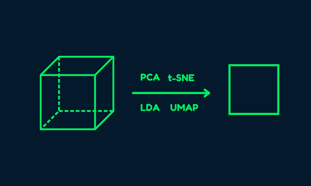
Image by Author
High-dimensional data, while rich in information, often contains redundant or irrelevant features. This can lead to several issues:
Dimensionality reduction addresses these issues by simplifying the data while retaining its most important features. This not only improves model performance but also makes the data easier to interpret and visualize.
Dimensionality reduction techniques can also be classified based on whether they assume a linear or nonlinear structure in the data.
Linear methods assume that the data lies in a linear subspace. These techniques are computationally efficient and work well when the data's structure is inherently linear.
Here are some examples:
Follow the Principal Component Analysis (PCA) in Python tutorial to learn how to extract information from data without supervision using the Breast Cancer and CIFAR-10 dataset.
Nonlinear methods are used when the data lies on a nonlinear manifold. These techniques are better suited for capturing complex structures in the data.
Here are some examples:
Dimensionality reduction techniques can be broadly categorized into two types: Feature selection and Feature extraction.
Feature selection involves identifying and retaining only the most relevant features from the dataset. This process does not transform the data but rather selects a subset of the original features.
Common methods include:
Feature extraction, also known as feature projection, transforms the data into a lower-dimensional space by creating new features that are combinations of the original ones. This approach is particularly useful when the original features are highly correlated or redundant.
Popular feature extraction methods include:
In this guide, we will learn how to apply dimensionality reduction techniques in Python.
We will start by importing the necessary Python packages and loading the digits dataset from sklearn.datasets.
import numpy as np
import matplotlib.pyplot as plt
from sklearn.datasets import load_digits
from sklearn.manifold import TSNE
from sklearn.preprocessing import StandardScaler


# Load the digits dataset
digits = load_digits()
X = digits.data   # shape (1797, 64)
y = digits.target # labels for digits (0 through 9)

print("Data shape:", X.shape)
print("Labels shape:", y.shape)
This dataset contains 1,797 grayscale images of handwritten digits (0–9), each represented as an 8x8 image (64 pixels). The data is flattened into a 64-dimensional feature vector for each image.
Data shape: (1797, 64)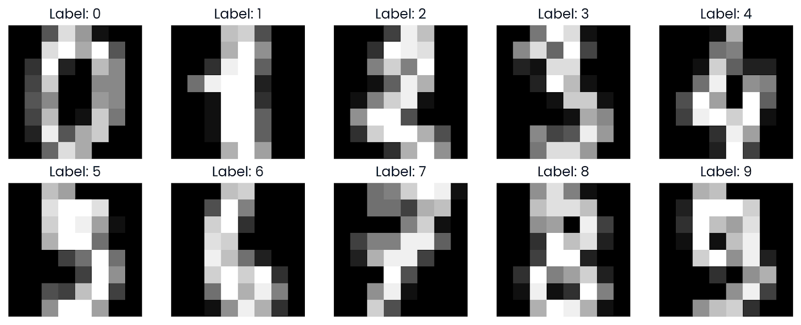
Labels shape: (1797,)We will now visualize a few samples from the dataset to gain a better understanding. Using Matplotlib, we will display images that have been reshaped back to their original 8x8 grid format.
def plot_digits(images, labels, n_rows=2, n_cols=5):
    fig, axes = plt.subplots(n_rows, n_cols, figsize=(10, 4))
    axes = axes.ravel()
    for i in range(n_rows * n_cols):
        axes[i].imshow(images[i].reshape(8, 8), cmap='gray')
        axes[i].set_title(f"Label: {labels[i]}")
        axes[i].axis('off')
    plt.tight_layout()
    plt.show()

plot_digits(X, y)
As we can see, it displays a grid of images, showing how the digits look in grayscale from 0 to 9.
t-SNE is a popular dimensionality reduction technique for visualizing high-dimensional data in 2D or 3D. It is particularly effective at preserving local structures in the data.
Read the blog Introduction to t-SNE: Nonlinear Dimensionality Reduction and Data Visualization to learn how to visualize high-dimensional data in a low-dimensional space using a nonlinear dimensionality reduction technique.
Before applying t-SNE, we scale the data using StandardScaler to normalize the feature values.
scaler = StandardScaler()
X_scaled = scaler.fit_transform(X)
Then, we select a subset of 500 samples for faster computation and run the t-SNE algorithm on the subset.
Here are the TSNE function’s arguments with explanation:
n_samples = 500
X_sub = X_scaled[:n_samples]
y_sub = y[:n_samples]

tsne = TSNE(n_components=2,
            perplexity=30,
            n_iter=1000,
            random_state=42)
X_tsne = tsne.fit_transform(X_sub)

print("t-SNE result shape:", X_tsne.shape)
The dimensionality reduction was successful, as we now have 500 samples, each represented in 2 dimensions.
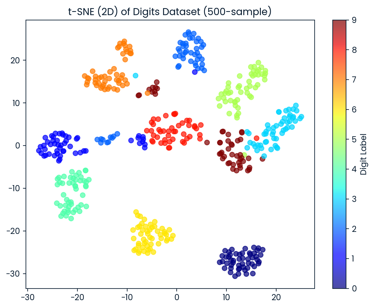
t-SNE result shape: (500, 2)We now visualize the 2D t-SNE dataset. Each point is colored based on its digit label, allowing us to observe how well t-SNE separates the different digit classes.
plt.figure(figsize=(8, 6))
scatter = plt.scatter(X_tsne[:, 0], X_tsne[:, 1],
                      c=y_sub, cmap='jet', alpha=0.7)
plt.colorbar(scatter, label='Digit Label')
plt.title('t-SNE (2D) of Digits Dataset (500-sample)')
plt.show()
The t-SNE effectively separated the digits into 10 distinct groups, with some overlapping between groups.
To explore the t-SNE space further, we randomly select two points and calculate the Euclidean distance between them in the 2D t-SNE space. We will also visualize the images to see how similar they are.
import random
idx1, idx2 = random.sample(range(X_tsne.shape[0]), 2)
point1, point2 = X_tsne[idx1], X_tsne[idx2]
dist_tsne = np.linalg.norm(point1 - point2)
print(f"Comparing images #{idx1} and #{idx2}")
print(f"Distance in t-SNE space: {dist_tsne:.4f}")
print(f"Label of image #{idx1}: {y_sub[idx1]}")
print(f"Label of image #{idx2}: {y_sub[idx2]}")
# Plot the original images
fig, axes = plt.subplots(1, 2, figsize=(6, 3))
axes[0].imshow(X[idx1].reshape(8, 8), cmap='gray')
axes[0].set_title(f"Label: {y_sub[idx1]}")
axes[0].axis('off')
axes[1].imshow(X[idx2].reshape(8, 8), cmap='gray')
axes[1].set_title(f"Label: {y_sub[idx2]}")
axes[1].axis('off')
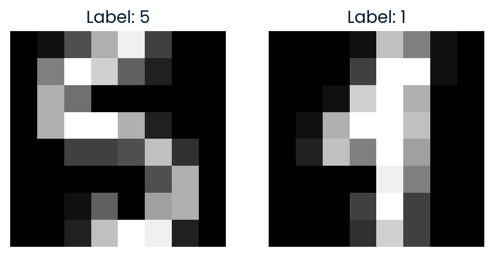
plt.show()The distance in t-SNE space reflects how dissimilar the two images are in the reduced 2D representation.
Comparing images #291 and #90
Distance in t-SNE space: 35.7666
Label of image #291: 5
Label of image #90: 1
If you are having trouble running the code above, please check the DataLab workspace for further assistance.
Dimensionality reduction plays a crucial role in real-world applications by improving the efficiency, accuracy, and interpretability of machine learning models, as well as enabling better visualization and analysis of complex datasets.
In this tutorial, we have explored the concept of dimensionality reduction, its purpose, methods, and types. Finally, we have learned how to use the t-SNE technique to transform image data into a lower-dimensional space for visualization and analysis.
Take the Dimensionality Reduction in Python course to Understand the concept of reducing dimensionality in your data and master the techniques for doing so in Python.
Top DataCamp Courses
Track
Track
Course
blog
Abid Ali Awan
7 min
blog
Kurtis Pykes
9 min
cheat-sheet
Joe Franklin
Tutorial
Abid Ali Awan
Tutorial
Samuel Shaibu
code-along
Matt Pickard