Unhide All Rows in Excel: Simple Tips, Shortcuts, and Fixes

You’re working in Excel when something feels off. The data looks fine at first glance, but some numbers aren’t adding up. You check the formulas, double-check the totals, and still can’t find the problem.

The rows aren’t deleted; they’re hidden. And if you don’t know how to spot them, you could miss important information without realizing it.

In this guide, I’ll show you several ways to unhide rows in Excel, from quick clicks and keyboard shortcuts to using VBA for more advanced cases. We’ll also cover common mistakes, troubleshooting steps, and best practices so you can keep your data clear and ready to work with.

Why Rows May Be Hidden in Excel 

Before you unhide rows, let’s understand why they’re hidden. Sometimes it’s intentional, other times it’s by accident, and the reason can change how you fix it.

Common reasons include:

• Manually hidden: You might have right-clicked the row and chosen Hide.
• Filters: Rows that don’t match a filter get hidden automatically.
• Grouping: Collapsed row groups won’t show their contents.
• Row height set to zero: The row is still there, but has no visible height.
• Imported data or formatting issues: Copying from another file can bring in hidden rows or formatting that hides them.

Core Methods for Unhiding Rows

Now that you know why rows might be hidden, let’s go through the main ways to bring them back.

Unhiding all rows at once

If you’re not sure where the hidden rows are, the quickest fix is to reset the whole sheet so everything is visible again.

1. Select the entire sheet by pressing Ctrl + A (Windows) or Command + A (Mac).

2. On Windows: Go to the Home tab > Format > Hide & Unhide > Unhide Rows.

3. On Mac: With the sheet selected, go to the Format menu in the top bar > Row > Unhide.

This method works well if your top rows are hidden and you can’t click them directly.

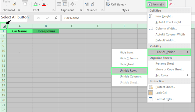
Unhide all the rows. Image by Author.

Keyboard shortcuts

Shortcuts are the fastest way to unhide rows if you use Excel on a daily basis.

1. Select the rows around the hidden ones or press Ctrl + A (Windows)/Command + A (Mac) to select the whole sheet.

2. Then, use the shortcut:

• Windows: Ctrl + Shift + 9

• Mac: Command + Shift + 9

This is ideal if you want to avoid using menus altogether.

Ribbon commands (Home tab)

If you prefer using Excel’s ribbon:

1. Select the rows around the hidden ones, or the entire sheet.
2. Go to the Home tab > Format > Hide & Unhide > Unhide Rows.

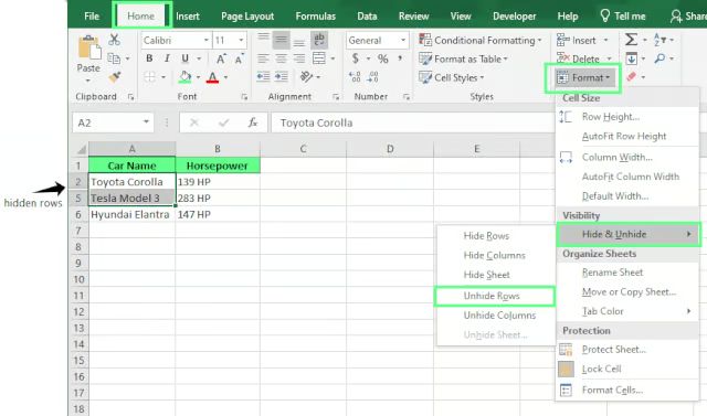
Unhide rows using the Excel Ribbon. Image by Author.

Context menu (right-click)

When you know exactly where the hidden rows are, do this:

1. Select the rows above and below the hidden ones.
2. Right-click the row number (not the cell).
3. Choose Unhide from the menu.

This method is perfect for unhiding one or two specific rows.

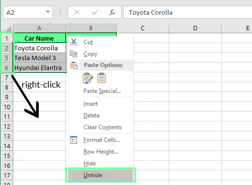
Unhide rows with the right-click option. Image by Author.

Double-clicking row headers

If you see a jump in row numbers (e.g., from 4 to 6), it means the row in between is hidden. To fix this:

1. Move your cursor to the line between the two visible row numbers until it turns into a double line with arrows.
2. Double-click that border to reveal the hidden row.

Note: This only works if the hidden rows are between visible ones. It won’t help if the first or last row is hidden.

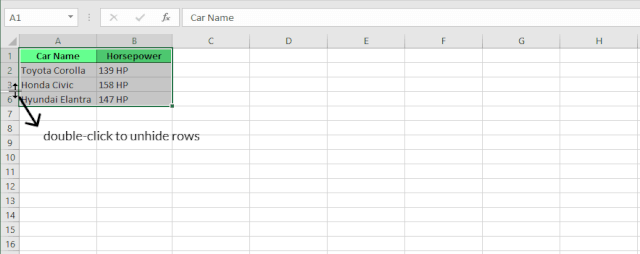
Unhide rows with a double-click. Image by Author.

Tip: If you select the whole column before double-clicking, Excel will unhide all the hidden rows in that column at once.

Advanced Techniques

If the usual methods don’t bring your rows back, Excel has a couple of more advanced options. But these are helpful if you work with large spreadsheets or want to automate the process.

VBA macros

VBA (Visual Basic for Applications) is Excel’s built-in programming tool. With just a few lines of code, you can unhide every row in a sheet. 

Here’s how to use it:

1. Press Alt + F11 (Windows) or Fn + Option + F11 (Mac) to open the VBA Editor.

2. In the menu, click Insert > Module.

3. Paste this code
   

Sub UnhideAllRows()
    Rows.Hidden = False
End Sub

4. Press F5 or click Run.

Every hidden row in your sheet will be visible again.

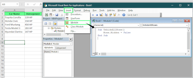
Unhide rows using VBA. Image by Author.

Grouping and outlines

Sometimes rows are hidden because they’re part of a group, not because someone manually hid them. Grouping is a feature in Excel that lets you collapse and expand sections of data. It’s quite useful for organization, but easy to overlook if you don’t use it often.

Here’s what to check:

• Look along the left edge of your sheet for plus (+) or minus (–) signs.
• Click a plus (+) sign to expand a group and show the rows inside.
• If rows are still missing, check for any collapsed groups elsewhere in the sheet.

Hidden vs. grouped rows: 

Hidden rows are made invisible manually. Grouped rows are collapsed as part of Excel’s outlining feature and can be expanded with the plus/minus controls.

Tip: To remove grouping completely, go to the Data tab and click Ungroup.

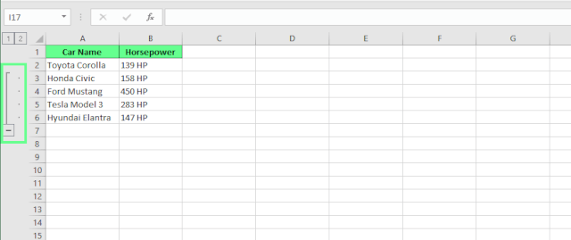
Ungroup to unhide the rows. Image by Author.

Troubleshooting Common Issues

Now, let’s look at a few issues that you may encounter when unhiding rows:

Rows with zero height

A row can look hidden if its height is set to zero, even if you didn’t hide it manually. So even if you right-click and choose Unhide, it won’t work in this case.

Here’s how to fix this:

1. Select the rows around the missing one.

2. Go to Home > Format > Row Height (or right-click the row number and choose Row Height).

3. Set the height to 15 (Excel’s default).

4. Click OK, and the row should appear again.

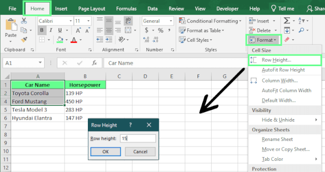
Adjust the row height. Image by Author.

Filtered rows

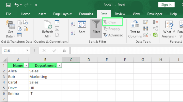
If your data is filtered, Excel will hide any rows that don’t meet the filter’s criteria. For example, if you filter by “Sales” in a Department column, only the “Sales” rows show; the others are hidden, even though they’re not deleted.

To confirm this, see if the color of row numbers changed. Because row numbers will turn blue when rows are filtered out.

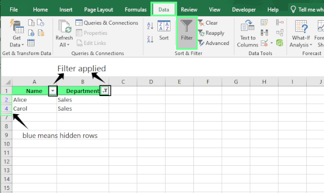
Rows got hidden when the filter was applied. Image by Author.

Here’s how to fix this:

1. Click anywhere in your table.
2. Go to the Data tab and click Clear to remove all filters.

Unhide rows by clearing filters. Image by Author. 

Protected or locked sheets

If the Hide and Unhide options are greyed out, the sheet is probably protected. And when protection is on, you can’t unhide rows until it’s removed.

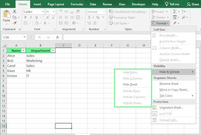
The Hide and Unhide option disabled. Image by Author.

Here’s how you can fix this:

1. Go to the Review tab.
2. Click Unprotect Sheet.
3. If a password prompt appears, enter the password.

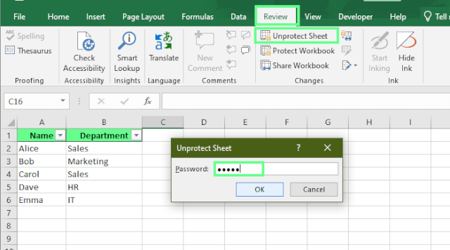
Unprotect the sheet and unhide the rows. Image by Author.

Tip: If you still want the sheet protected but need to hide/unhide rows, click Protect Sheet in the Review tab and check Format rows and Format columns before enabling protection.

Conflicting keyboard shortcuts

If Ctrl + Shift + 9 (Windows) or Command + Shift + 9 (Mac) isn’t working, another app or your system might be using that shortcut.

Here’s how you can fix this:

• Use the menu method: Home > Format > Unhide Rows.
• Check your Mac/Windows keyboard shortcut settings.
• Close any apps that might override Excel shortcuts (like screen recorders or custom hotkey tools).

Best Practices For Unhiding Rows

Here are a few habits that can save you from mistakes and keep your Excel sheets clean and easy to work with.

Select visible cells only

By default, Excel copies everything in your selection, even hidden rows. That means if rows 2–5 are hidden and you select rows 1, 6, and 7, Excel still pastes rows 2–5 in between.

To avoid this, here’s how you can copy only visible cells:

1. Select the range you want to copy.

2. Press Alt + ; (Windows) or Command + Shift + Z (Mac) to select only the visible cells.

3. Press Ctrl + C (Windows) or Command + C (Mac) to copy, then paste as usual.

This way, hidden rows stay hidden in your pasted data.

Use Go To Special to find hidden rows

When you work with a big dataset, it can be hard to identify where rows are hidden.  But the Go To Special feature makes it easy to find them.

Here’s how you can use this:

1. Go to Home > Find & Select > Go To Special. Or press F5 or Ctrl + G (Windows) to open Go To, then click Special.

2. Select Visible cells only and click OK.

Any gaps in the white selection border show where rows are hidden.

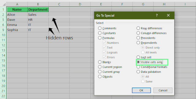
Find the hidden rows using the Go To Special tool. Image by Author.

Prevent accidental hiding and double-checking

Here are a few tips to avoid hiding rows by mistake and to manage your worksheet layout better:

• Be careful when selecting rows—a stray right-click or shortcut can hide them without you noticing.
• Use Freeze Panes (under the View tab) to keep headers or important rows in sight.
• If you use grouping, make sure it’s intentional and clearly labeled.
• Before printing or sending a file, take a minute to check for hidden rows.

Final Thoughts 

Hidden rows can throw off your data, but now you know exactly how to spot and unhide them.

If one method doesn’t work, check for filters, zero-height rows, grouping, or sheet protection. Once they’re visible again, take a minute to prevent it from happening in the future with Freeze Panes, clear grouping labels, and tidy sheet layouts.

So the next time rows “disappear,” you’ll know they’re not lost; they’re hidden, and only a couple of clicks away.

If you want to learn more about hiding and unhiding rows or columns in Excel, check out our guides on how to unhide columns and remove blank rows to keep your sheet clean and organized.