Lognormal Distribution: Definition, Properties, and Applications

Think about income data. A few people earn millions, most earn somewhere in the middle, and the distribution has a long tail stretching to the right. Plot it against a standard bell curve and nothing lines up because the normal distribution is a poor fit.

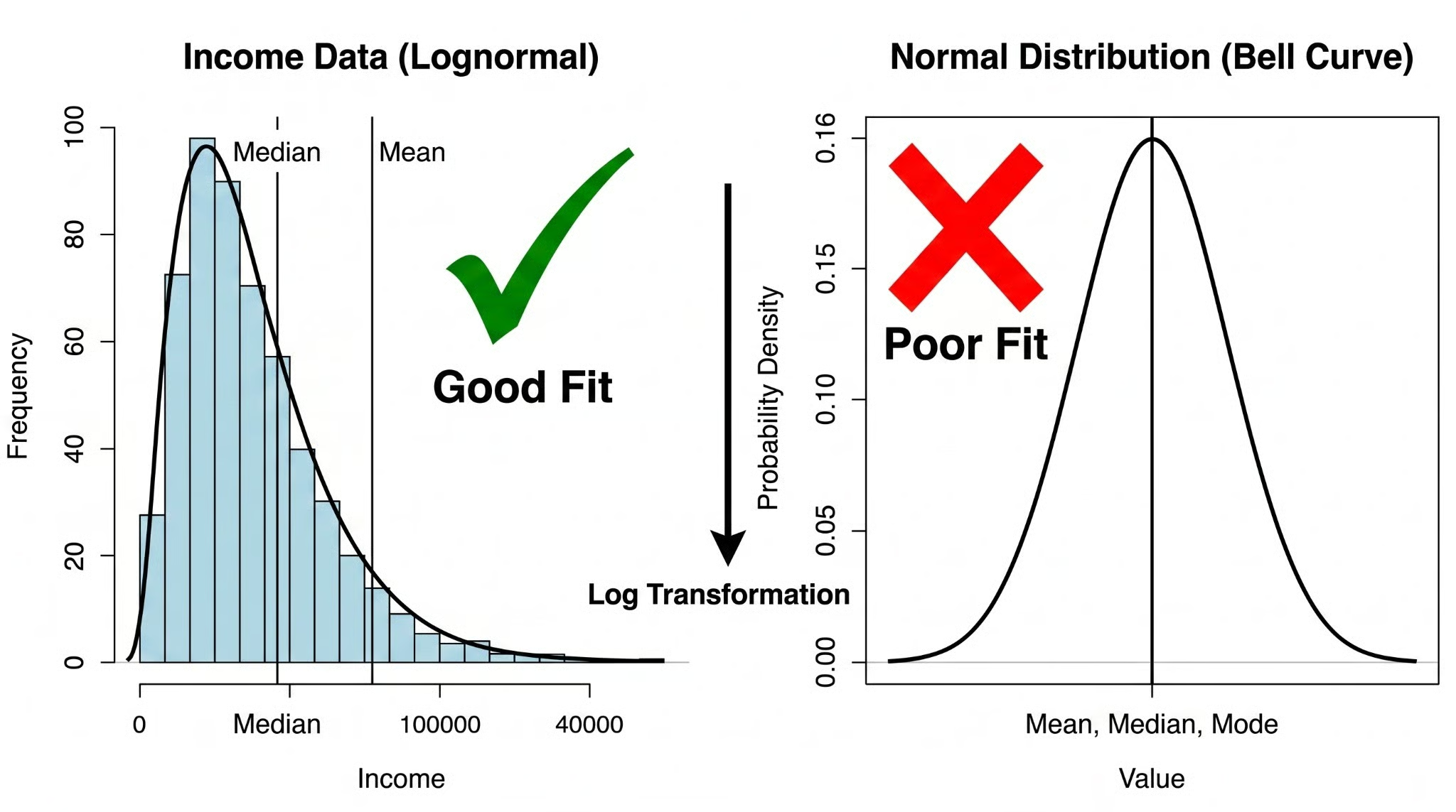
The lognormal distribution is built for variables that are strictly positive and right-skewed, where the spread grows with the size of the value. Household income, stock prices, file sizes, and biological measurements all behave this way.

We'll cover what the lognormal distribution is, how it compares to the normal distribution, its key properties and formula, when to use it, and how to spot it in real data, including some common mistakes.

What Is the Lognormal Distribution?

A random variable follows a lognormal distribution if its natural logarithm is normally distributed.

If X is lognormally distributed, then ln(X) is normal. The name comes directly from this: log-normal, a distribution whose log is normal.

Two things follow immediately. First, values are always positive. Logarithms are only defined for positive numbers, so lognormal variables can never be zero or negative. Second, the distribution is right-skewed. There's a physical lower bound at zero but no upper bound, which means the right tail stretches out much further than the left.

The logarithm transformation is the key connecting the two distributions. Take a lognormally distributed variable, apply a natural log to every observation, and the result is normally distributed data. This is more than a mathematical curiosity. It's what makes the lognormal tractable. All the statistical machinery built for the normal distribution becomes available once you've transformed your data.

Lognormal Distribution vs. Normal Distribution

The most immediate difference is shape. The normal distribution is symmetric, with its mean, median, and mode all at the same center point. The lognormal distribution is asymmetric, skewed to the right, with a long right tail. The mean, median, and mode are all different. We'll get to why in the next section.

The range of possible values differs too. A normal distribution extends from negative infinity to positive infinity. A lognormal distribution is bounded below by zero and extends upward without limit. This makes it the right model whenever your variable physically can't be negative.

That last row matters most in practice. Taking the logarithm of a lognormally distributed variable produces a normal distribution. This transformation is what makes the lognormal useful. It's not just a description of skewed data, it's a model with a direct bridge back to the normal world.

Properties of the Lognormal Distribution

There are couple key properties of a lognormal distribution that make it special. 

Always positive with a long right tail

The lognormal distribution produces only positive values. If ln(X) is normal, then X = e^(ln(X)) is always positive, since exponentials are always positive. There's a floor at zero, but no ceiling. Combined with the right skew, this gives the distribution its characteristic shape: a sharp rise from zero, a peak somewhere to the left of the mean, then a long tapering tail.

Mean, median, and mode are all different

The three measures of the center tell different stories. The mode (the most common value) sits furthest to the left. The median (the middle value) is higher. The mean (the arithmetic average) is higher still, pulled upward by the right tail. In income data, mean household income is substantially higher than the median. A few very high earners shift the average while leaving the middle of the distribution untouched. This is why economists typically report median income when describing typical households. Choosing the wrong measure of center here isn't just sloppy statistics; it actively misleads.

Keep this in mind when we reach the formula: μ and σ describe the underlying normal distribution of ln(X), not the mean and standard deviation of X itself. That distinction catches many people off guard.

The Lognormal Distribution Formula

The probability density function (PDF) of the lognormal distribution is:

for x > 0, where:

• x is the value of the random variable (must be positive)
• μ (mu) is the mean of ln(X). It controls the location of the distribution—shifting μ up moves the peak rightward.
• σ (sigma) is the standard deviation of ln(X). It controls the spread and degree of skew. A larger σ produces a heavier right tail.

μ and σ are not the mean and standard deviation of X itself. They're the parameters of ln(X). The actual mean of X is e^{(μ + σ²/2)}, which is why it sits to the right of the median. If you're fitting a lognormal to data in Python or R, the library functions handle this translation for you, but it's worth knowing what the parameters actually represent.

When Should You Use a Lognormal Distribution?

The practical test: if your variable is strictly positive and the growth process is multiplicative rather than additive, the lognormal is likely a good fit.

Additive processes tend to produce normal distributions. By the central limit theorem, sums of many small random effects converge to normal. Multiplicative processes are different. When each period's value is the previous value multiplied by a random factor (compound interest, bacteria doubling), the result over many periods is lognormal. This is why the lognormal appears so often in finance and biology.

The lognormal fits variables like:

• Financial returns over long horizons—daily log returns compound multiplicatively
• Insurance claims—most are small; a few are very large
• Income distributions—bounded below by zero, right-skewed in practice
• Biological growth—organism size, cell counts, concentration measurements
• Waiting times—repair times and service durations with occasional outliers
• Environmental measurements—pollutant concentrations in water or air

If you're unsure whether the lognormal is appropriate, our Feature Engineering for Machine Learning in Python course covers log transformations in depth, including how to assess whether a transformation suits your data.

Real-World Examples of the Lognormal Distribution

The lognormal distribution appears in many real-world scenarios, few of which are highlighted below. 

Income and wealth

Income data is the textbook lognormal example. Most people earn incomes clustered in a moderate range, but there's no upper bound—a small number of individuals earn orders of magnitude more than the median. Plot raw household income and you get a sharply right-skewed histogram; take the log and it looks roughly normal. Wealth data shows the same pattern, often with a more pronounced skew.

Stock prices

Daily stock price changes are approximately normally distributed in log terms, which means the price level itself follows a lognormal distribution over time. This assumption underlies the Black-Scholes option pricing model. Stock prices can't go below zero, they compound multiplicatively, and they produce that characteristic right tail.

Internet file sizes

File sizes span an enormous range, from a few kilobytes to many gigabytes, and the distribution is heavily right-skewed. The lognormal fits well here because file size is bounded below by zero and grows multiplicatively. Web traffic analysis and network engineering rely on this.

Biological measurements

Concentrations of biological substances (hormone levels, pollutant concentrations in tissue, microbial counts) tend to follow lognormal distributions. Biological processes often involve ratios and growth rates rather than additive increments. Latency times in medical studies show the same pattern.

In each of these domains, the logic is the same: a process that's multiplicative in nature, bounded at zero, and capable of producing rare extreme values is a natural candidate for lognormal modeling.

Lognormal Distribution in Machine Learning and Data Science

The lognormal distribution shows up in machine learning in a few distinct ways, each requiring slightly different handling.

Modeling positive continuous variables

When a target variable is strictly positive and right-skewed—housing prices, revenue, user lifetime value—applying a log transformation before modeling often improves results substantially. Linear regression assumes normally distributed residuals; fitting it to raw lognormal data violates that assumption. The fix: log the target, fit the model, then exponentiate predictions back to the original scale. One caveat: interpreting coefficients in log-space requires care, since a unit increase in a predictor now corresponds to a multiplicative change in the original scale.

Feature engineering with log transformations

Log-transforming skewed features before feeding them to scale-sensitive models (linear regression, logistic regression, k-means) reduces the influence of extreme values and makes relationships more linear. This is standard preprocessing for right-skewed continuous features. The transformation also handles outliers implicitly: a value that's 100 times the median in raw space becomes roughly 4.6 units above the median in log space.

Probabilistic modeling and simulation

Some probabilistic models use the lognormal distribution explicitly. In Bayesian modeling, it's a common prior for parameters that must be positive. In simulation, it models quantities like repair times, insurance claim sizes, and network delays where the multiplicative structure matches real-world processes. These appear regularly in applied work.

How to Identify a Lognormal Distribution

Eyeballing a histogram isn't enough. Here are the approaches that actually work, in roughly increasing order of rigor.

Histogram and log-transformed histogram

Start with a histogram of the raw data. If it's right-skewed with a long right tail and a lower bound near zero, that's suggestive. Then plot a histogram of the log-transformed values. If that histogram looks approximately symmetric and bell-shaped, the lognormal is a plausible model. This two-plot comparison is fast. But don't stop here.

Q-Q plots

A quantile-quantile (Q-Q) plot compares the quantiles of your data against the quantiles of a theoretical distribution. For lognormal data, plot the quantiles of ln(X) against the quantiles of a standard normal. Points falling approximately along a straight line indicate a good fit. Systematic curvature, especially in the tails, suggests the lognormal isn't quite right. Our tutorial on Q-Q plots covers how to read and interpret them in both Python and R.

Goodness-of-fit tests

For a formal test, apply a normality test (Shapiro-Wilk, Kolmogorov-Smirnov, Anderson-Darling) to the log-transformed data. If ln(X) passes, you have statistical evidence supporting the lognormal model. With very large datasets, though, these tests become sensitive enough to reject lognormality for trivially small deviations. Always pair formal tests with visual inspection.

Using all three approaches together gives you a much more reliable picture than any single method alone.

Common Mistakes When Working With Lognormal Data

A few common errors that many practitioners often make are highlighted here. 

Assuming the data is normally distributed

This is the most common error. Fitting a normal distribution to lognormal data understates the probability of extreme values, biases estimates of the mean, and can make statistical tests unreliable. If your data is positive and right-skewed, check before reaching for the normal distribution.

Interpreting the arithmetic mean incorrectly

For lognormal data, the arithmetic mean is pulled substantially above the median by the right tail. Reporting the mean as "typical" is misleading. The median is usually the better measure of what a typical observation looks like. Be clear about which measure you're reporting and why.

Forgetting that values must be positive

The lognormal distribution is undefined for zero or negative values. If your dataset contains zeros—common in count data or sales data with inactive periods—the lognormal isn't directly applicable. Common workarounds include adding a small constant before logging (not ideal statistically) or using a zero-inflated model that handles the zeros separately.

Applying inappropriate statistical tests

Tests designed for normally distributed data (t-tests, standard confidence intervals, ANOVA) don't directly apply to lognormal data. You have two options: log the data and apply normal-based methods, or use non-parametric methods that make no assumptions about shape. The wrong test won't always produce dramatically wrong answers, but it can produce subtly biased ones that are hard to detect.

Conclusion

The lognormal distribution models positive, right-skewed variables by connecting them to the normal distribution through a logarithm transformation. Once you recognize that ln(X) is normal whenever X is lognormal, the rest follows. You can work in log-space using standard normal tools, then translate results back to the original scale.

We've covered the distribution's key properties, traced them back to that transformation, and looked at where it appears in practice. The practical takeaway is straightforward: before modeling positive, right-skewed data, check for lognormality. Plot the log-transformed data, run a normality test on it, and look at a Q-Q plot. Our Introduction to Statistics in Python course and Probability Distributions in Python tutorial are good next steps if you want to see these ideas applied to real datasets.