Course
Machine Learning with Tree-Based Models in Python
5 hr
116.3K
Today, many large organizations use some form of predictive modeling to maximize revenue and drive business growth.
Machine learning has a variety of use-cases in different domains. Subscription-based platforms like Netflix and Spotify, for instance, use machine learning to recommend content based on user activity on the application.
Recommendation systems add direct business value to these companies since a better user experience will make it likely for customers to continue subscribing to the platform. This is an example of an unsupervised machine learning model.
Similarly, a mobile service provider might use machine learning to analyze user sentiment and curate its product offering according to market demand. This is an example of a supervised machine learning model.
All machine learning models can be classified as supervised or unsupervised. The biggest difference between the two is that a supervised algorithm requires labeled input and output training data, while an unsupervised model can process raw, unlabeled datasets.
Supervised machine learning models can then be further classified into regression and classification algorithms, which will be explained in more detail in this article.
Regression algorithms are used to predict a continuous outcome (y) using independent variables (x).
For example, look at the table below:
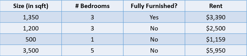
Image by author
In this case, we would like to predict the rent of a house based on its size, the number of bedrooms, and whether it is fully furnished. The dependent variable, “Rent”, is numeric, which makes this a regression problem.
A problem with many input variables like the one above is called a multivariate regression problem.
A common misconception by data science beginners is that a regression model can be evaluated using a metric like accuracy. Accuracy is a metric used to assess the performance of classification models, as will be explained later in this article.
Regression models, on the other hand, are evaluated using metrics such as MAE (Mean Absolute Error), MSE (Mean Squared Error), and RMSE (Root Mean Squared Error).
Let’s add a predicted value to the house price problem above and evaluate these predictions using a few regression metrics:
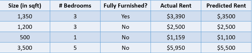
Image by author
The mean absolute error calculates the sum of the difference between all true and predicted values, and divides this by the total number of observations. Here is the formula to calculate MAE:
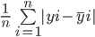
Let’s calculate the Mean Absolute Error of the above values using this formula:
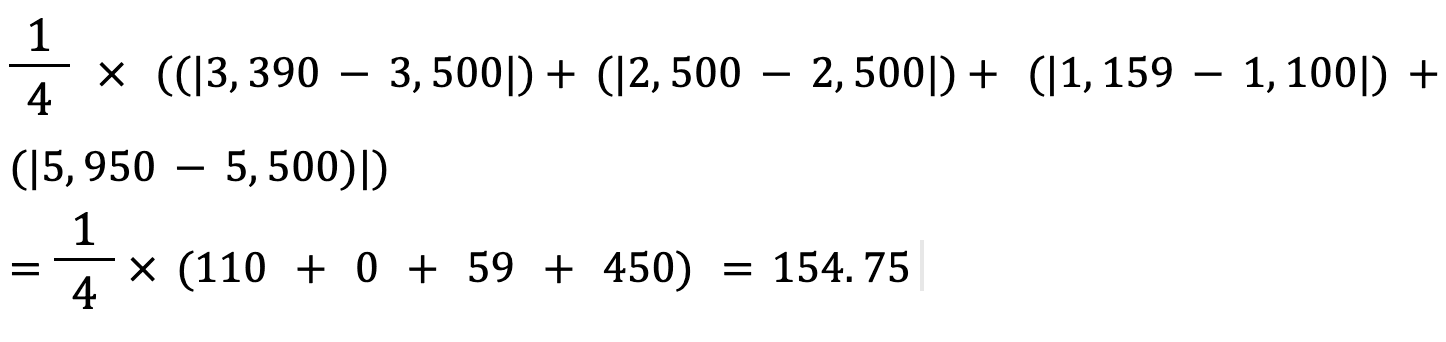
The mean absolute error between the actual and predicted house price is approximately $155.
The formula to calculate a model’s mean squared error is similar to that of its mean absolute error:
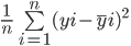
Note that while the mean absolute error calculates the average absolute distance between the actual and predicted value, the mean squared error finds the averaged squared distance between actual and predicted values.
Let’s calculate the MSE between the actual and predicted values above:
The RMSE of an estimator is calculated by finding the square root of its mean squared error. One advantage of calculating a dataset’s RMSE over its MSE is that the error is returned in the same unit of the variable we are predicting.
In this case, for instance, the RMSE is √54,520.25=233.5. This value is interpretable since it is in terms of house price, while the Mean Squared Error was not.
Now that you understand the concept of regression, let’s look into the different types of regression models:
Linear regression is a linear approach to modeling the relationship between a dependent and one or more independent variables. This algorithm involves finding a line that best fits the data at hand.
Here is a visual representation of how a simple linear regression model works:
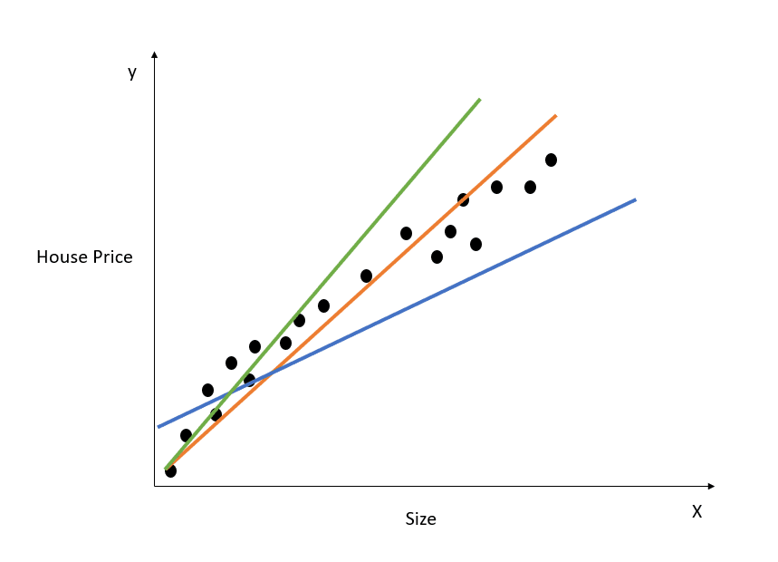
Image by author
The chart above showcases the relationship between house price and size. The linear regression model will create a line that best models this relationship. All house price predictions relative to different values of size will lie on the best fit line.
Observe that there are three lines drawn on the diagram above. Which of these lines is the “line of best fit?”
Just by looking at the diagram above, we can see that the orange line is the closest to all the data points showcased. Hence, we can intuitively say that it represents the “line of best fit.”
Here is a more formal explanation as to how the line of best fit is found in linear regression:
The equation of a straight line is y=mx+c. Here, m represents the slope of the line and c represents its y intercept. There are infinite ways to draw this line, as there are infinite possible values for m and c.
The line of best fit, also known as the least squares regression line, is found by minimizing the sum of squared distance between the true and predicted values:

You can read the Essentials of Linear Regression in Python tutorial to gain a deeper understanding of the linear regression machine learning model and its implementation.
Ridge regression is an extension of the linear regression model explained above. It is a technique used to keep a regression model’s coefficients as low as possible.
One problem with a simple linear regression model is that its coefficients can become large, which makes the model more sensitive to inputs. This can lead to overfitting.
Let’s take a simple example to understand the concept of overfitting:
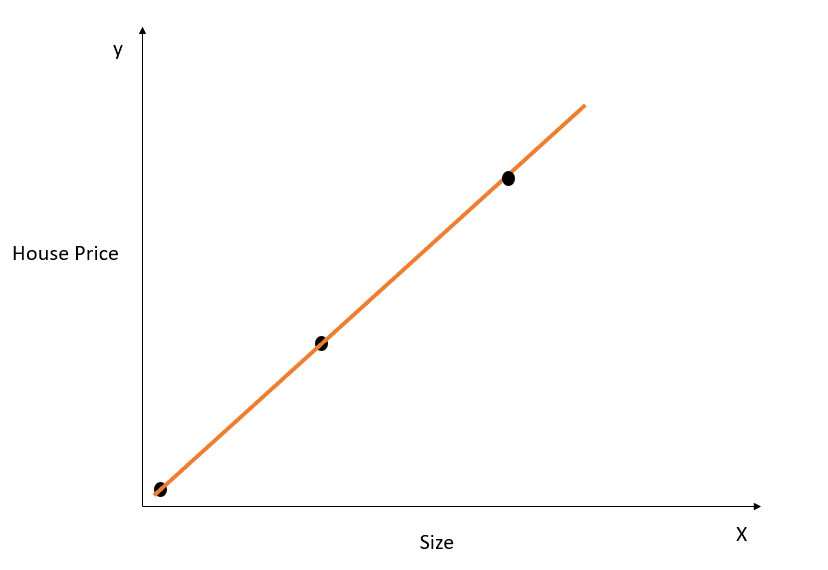
Image by author
In the figure above, the line of best fit above models the relationship between X and y perfectly, and the sum of squared distance between the true and predicted values is 0. Recall that the equation for this line is y=mx+c.
While this line is a perfect fit on the training dataset, it likely would not generalize well to test data. This phenomenon is called overfitting, and you can read this article on overfitting to learn more about it.
In simple words, a model that is highly complex will pick up on unnecessary nuances of the training dataset that aren’t reflected in the real world. This model will perform extremely well on training data but will underperform on datasets outside what it was trained on.
A linear regression model with large coefficients is prone to overfitting.
Ridge regression is a regularization technique that will force the algorithm to choose smaller coefficients by penalizing its loss function to include an additional cost.
As shown in the previous section, here is the error that we want to minimize in simple linear regression:
In ridge regression, this equation will change slightly, and a penalty term will be added to the above error:

Notice that there is a value (lambda) multiplied to the model’s coefficients. Since this model only has one variable, there is a single coefficient with a penalty term added to it. If there are multiple independent variables, lambda will be multiplied by the sum of squared coefficients.
This penalty term punishes the model for choosing larger coefficients. The aim here is to shrink the coefficient values so that variables with a minor contribution to the outcome will have their coefficients close to 0. This reduces model variance and helps mitigate overfitting.
Observe that a lambda value of 0 will have no effect whatsoever, and the penalty term is eliminated. A higher value of lambda will add a larger shrinkage penalty, and the model coefficients will get closer to zero.
When choosing a lambda value, make sure to strike a balance between simplicity and a good training data fit. A higher lambda value results in a simple, generalized model, but choosing a value that is too high comes with the risk of underfitting. On the other hand, choosing a value of lambda that is very close to zero can lead to a highly complex model.
Lasso regression is another extension of linear regression that shrinks model coefficients by adding a penalty term to its cost function.
Here is the error that needs to be minimized in lasso regression:

Notice that this equation is like that of a ridge regression model, except, instead of multiplying lambda to the square of the coefficient, we are multiplying it with the coefficient’s absolute value.
The biggest difference between ridge and lasso regression is that in ridge regression, while model coefficients can shrink towards zero, they never actually become zero. In lasso regression, it is possible for model coefficients to become zero.
If an independent variable’s coefficient reaches zero, the feature can be eliminated from the model. This reduces the feature space and makes the algorithm easier to interpret, which is the biggest advantage of lasso regression.
Due to this, lasso regression can also be used as a feature selection technique, since variables with low importance can have coefficients that reach zero and will be removed entirely from the model.
You can build linear, ridge, and lasso regression models using the Scikit-Learn library:
1. Linear Regression
from sklearn.linear_model import LinearRegression
lr_model = LinearRegression()
To fit the model on your training dataset, run:
lr_model.fit(X_train,y_train)2. Ridge Regression
from sklearn.linear_model import Ridge
model = Ridge(alpha=1.0)
The lambda term can be configured via the “alpha” parameter when defining the model.
3. Lasso Regression
from sklearn.linear_model import Lasso
model = Lasso(alpha=1.0)
If you’d like to learn more about linear models and how to build them in Python, take our Introduction to Linear Modeling in Python course.
We use Classification algorithms to predict a discrete outcome (y) using independent variables (x). The dependent variable, in this case, is always a class or category.
For example, predicting whether a patient is likely to develop heart disease based on their risk factors is a classification problem:
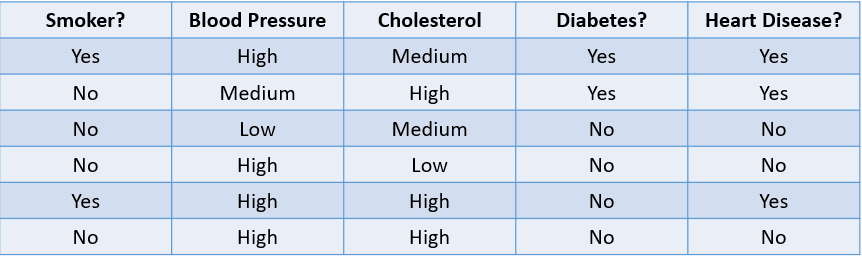
Image by author
The table above showcases a classification problem with four independent variables and one dependent variable, heart disease. Since there are only two possible outcomes (Yes and No), this is called a binary classification problem.
Other examples of a binary classification problem include classifying whether an email is spam or legitimate, customer churn prediction, and deciding whether to provide someone a loan.
A multiclass classification problem is one with three or more possible outcomes, such as weather forecasting or distinguishing between different animal species.
There are many ways to evaluate a classification model. While accuracy is the most used metric, it is not always the most reliable.
Let’s look at some common methods used to evaluate a classification algorithm based on the dataset below:
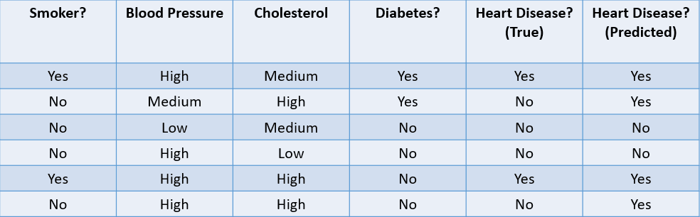
Image by author
1. Accuracy: Accuracy can be defined as the fraction of correct predictions made by the machine learning model.
The formula to calculate accuracy is:

In this case, the accuracy is 46, or 0.67.
2. Precision: Precision is a metric used to calculate the quality of positive predictions made by the model. It is defined as:

The above model has a precision of 24, or 0.5.
3. Recall: Recall is used to calculate the quality of negative predictions made by the model. It is defined as:

The above model has a recall of 2/2 or 1.
Let’s look at a simple example to understand the difference between precision and recall:
There is a rare, fatal disease that affects a fraction of the population. 95% of the patients in a hospital’s database do not have the disease, while only 5% do. If we build a machine learning algorithm that predicts that nobody has the disease, then the training accuracy of this model will be 95%. Despite the high accuracy, we know this is not a good model since it fails to identify patients with the disease.
This is where metrics like precision and recall come in. Precision, or specificity, tells us the ability of the model to correctly identify people without the disease. Recall, or sensitivity, tells us how well the model identifies people with the disease.
A “good” precision and recall value is subjective and depends on your use case.
In this disease prediction scenario, we always want to identify people with the disease, even if this comes with the risk of a false positive. Here, we will build the model to have higher recall than precision.
On the other hand, if we were to build a model that prevents malicious actors from entering an e-commerce website, we might want higher precision since blocking legitimate users will lead to a decline in sales.
We often use a metric called the F1-Score to find the harmonic mean of a classifier’s precision and recall. Simply put, the F1-Score combines precision and recall into a single metric by computing their average.
AUC, or Area Under the Curve, is another popular metric used to measure the performance of a classification model. An algorithm’s AUC tells us about its ability to distinguish between positive and negative classes.
To learn more about measures like AUC and how they are calculated, take the Supervised Learning in R course by Datacamp.
Now, let’s look at the different types of classification models and how they work:
Logistic regression is a simple classification model that predicts the probability of an event taking place.
Here is an example of how the logistic regression model works:
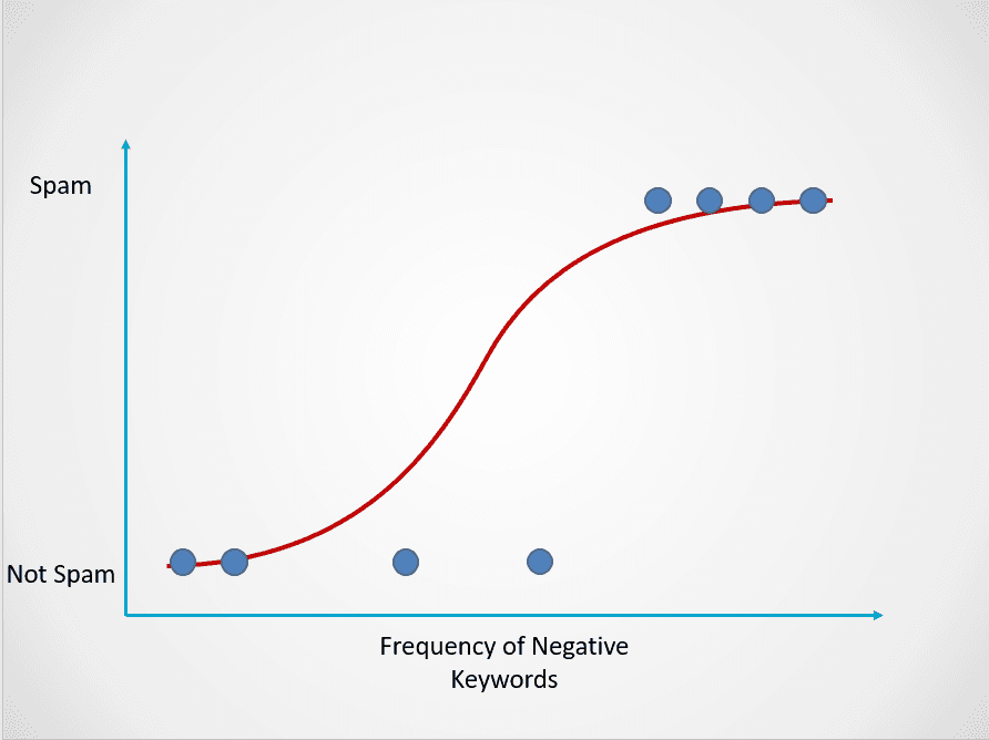
Image by author
The chart above displays a logistic function that maps email data into two categories: “Spam” and “Not Spam” based on the frequency of negative keywords in its text.
Observe that, unlike the linear regression algorithm, logistic regression is modeled with an S-shaped curve. This is known as the logistic function and has the following formula:
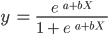
While the linear function does not have an upper and lower bound, the logistic function ranges between 0 and 1. The model predicts a probability that ranges from 0 to 1, which determines the class that the data point belongs to.
In this spam email example, if the text contains little to no suspicious keywords, then the probability of it being spam will be low and close to 0. On the other hand, an email with many suspicious keywords will have a high probability of being spam, close to 1.
This probability is then turned into a classification outcome:
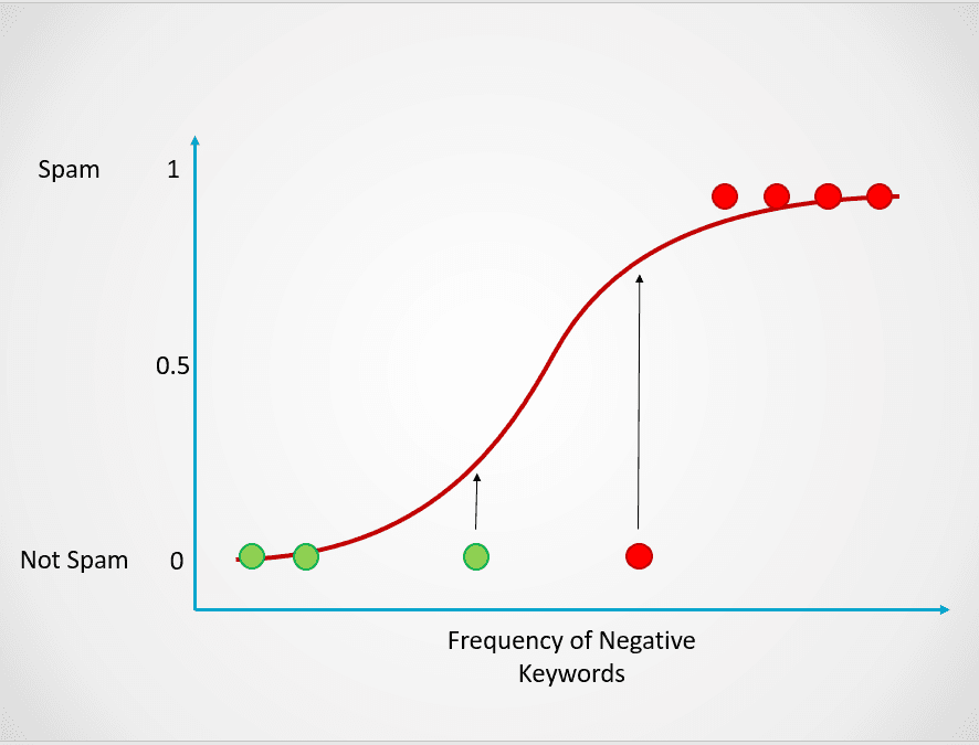
Image by author
All the points colored in red have a probability >= 0.5 of being spam. Hence, they are classified as spam and the logistic regression model will return a classification outcome of 1. The points colored in green have a probability < 0.5 of being spam, so they are classified by the model as “Not Spam” and will return a classification outcome of 0.
For binary classification problems like the above, the default threshold of a logistic regression model is 0.5, which means that data points with a higher probability than 0.5 will automatically be assigned a label of 1. This threshold value can be manually changed depending on your use case to achieve better results.
Now, recall that in linear regression, we found the line of best fit by minimizing the sum of squared error between the predicted and true values. In logistic regression, however, the coefficients are estimated using a technique called maximum likelihood estimation instead of least squares.
Read Python logistic regression tutorial to learn more about the concept of maximum likelihood estimation and how logistic regression works.
KNN is a classification algorithm that classifies a data point based on what group the data points nearest to it belong to.
Here is a simple example to demonstrate how the K-Nearest Neighbors model works:
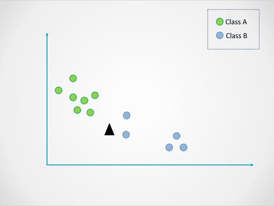
Image by author
In the diagram above, there are two classes of data points - A and B. The black triangle represents a new data point that needs to be classified into one of these two classes.
The K-Nearest Neighbors algorithm works like this:
In the visual above, the value of k is 1. This means that we look at only one closest neighbor to the black triangle and assign the data point to that class. The new data point is closest to the blue point, so we assign it to class B.
Now, let’s amend the value of k. Let’s try two possible values of k, 3 and 7:
Image by author
Now, notice that when we choose k=3, the new data point is between two categories. This means that we pick the majority class. Tw nearest neighbors are blue, and one nearest neighbor is green, so the data point will again be assigned to the class with blue points, class B.
When k=7, however, things change. Now, two nearest neighbors are blue, and seven are green. In this case, the data point will be assigned to the green class, class A.
Choosing different values of k will impact what class the new point is assigned to.
Selecting a value that is too small can be noisy and subject to outliers while selecting a large value might make you overlook categories with fewer data points.
If you’d like to learn more about the K-Nearest Neighbors algorithm and how to select an optimal “k” value, read this KNN tutorial.
Here are some code snippets you can use to build a classification model in Python using the Scikit-Learn library:
1. Logistic Regression
from sklearn.linear_model import LogisticRegression
log_reg = LogisticRegression()
2. K-Nearest Neighbors
from sklearn.neighbors import KNeighborsClassifier
knn = KNeighborsClassifier()Tree-based models are supervised machine learning algorithms that construct a tree-like structure to make predictions. They can be used for both classification and regression problems.
In this section, we will explore two of the most commonly used tree-based machine learning models: decision trees and random forests.
A decision tree is the simplest tree-based machine learning algorithm. This model allows us to continuously split the dataset based on specific parameters until a final decision is made.
Here is a simple example demonstrating how the decision tree algorithm works:
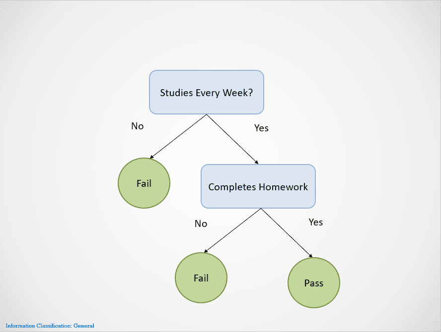
Image by author
Decision trees split on different nodes until an outcome is obtained.
In this case, if a student does not study every week, they will fail. If they study every week but do not complete their homework, the result is still “Fail.” They will only pass if they were to study every week and finish all their homework.
Notice that the decision tree above splits first on the variable “Studies Every Week?” It then stops splitting if the answer is “No,” saying that the student will fail.
The decision tree will choose a variable to split on first based on a metric called entropy. It will stop splitting when a “pure split” is obtained, i.e., when all the data points belong to a single class.
There are many ways to build a decision tree. The tree needs to find a feature to split on first, second, third, etc. This structure is created based on a metric called information gain. The best possible decision tree is one with the highest information gain.
To learn more about how decision trees work, along with metrics like entropy and information gain, this Python decision tree classification article has more details.
One of the biggest advantages of decision trees is that they are highly interpretable. It is easy to work backward and understand how a decision tree has obtained its final outcome based on the training dataset.
However, decision trees are also highly prone to overfitting if left to grow completely. This is because they are designed to split perfectly on all samples of the training dataset, which makes them unable to generalize well to external data.
This drawback of decision trees can be solved by using the random forest algorithm.
The random forest model is a tree-based algorithm that helps us mitigate some of the problems that arise when using decision trees, one of which is overfitting. Random forests are created by combining the predictions made by multiple decision tree models and returning a single output.
It does this in two steps:
In case of a regression problem, the outcome will be the average prediction of all decision trees.
Here is a simple visual to showcase how the random forest algorithm works:
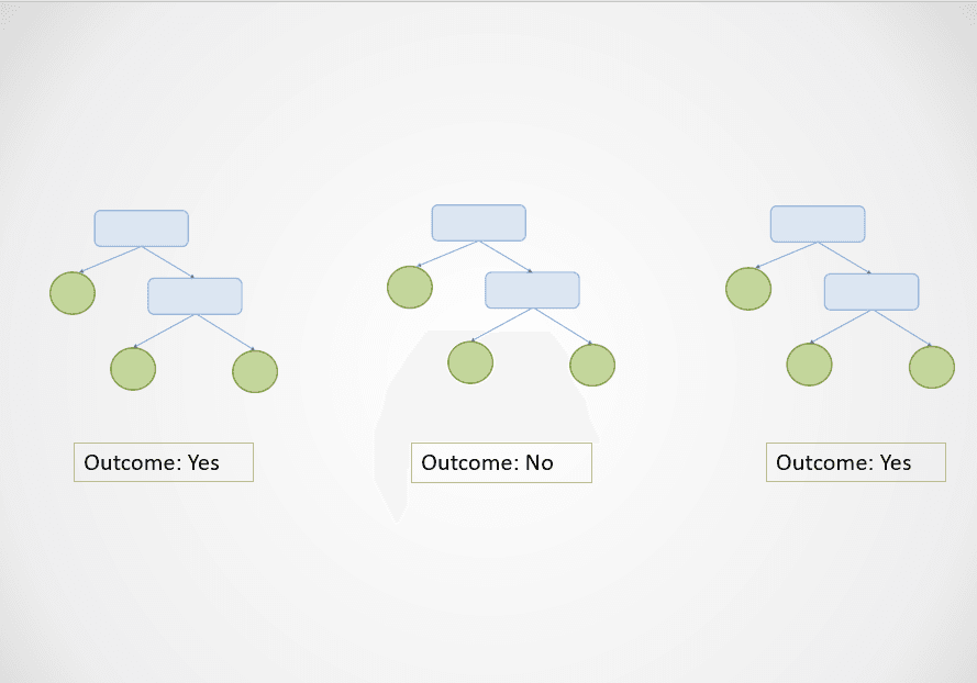
Image by author
In the diagram above, the first and third decision trees predict “Yes” while the second predicts “No.”
Since this is a classification task, the majority class is selected. In this case, the random forest algorithm will return a final outcome of “Yes” based on the predictions made by 2 out of 3 decision trees.
One of the biggest advantages of the random forest algorithm is that it generalizes well, since it combines the output of multiple decision trees that are trained on a subset of features.
Furthermore, while the output of a single decision tree can vary dramatically based on a small change in the training dataset, this problem does not arise with the random forest algorithm as the training dataset is sampled many times.
Run the following lines of code to build a tree-based machine learning algorithm with Scikit-Learn:
1. Decision Tree
# classification

from sklearn.tree import DecisionTreeClassifier
clf = DecisionTreeClassifier()

# regression

from sklearn.tree import DecisionTreeRegressor
dt_reg = DecisionTreeRegressor()
2. Random Forests
# classification

from sklearn.ensemble import RandomForestClassifier
rf_clf = RandomForestClassifier()

# regression

from sklearn.ensemble import RandomForestRegressor
rf_reg = RandomForestRegressor()So far, we’ve explored supervised machine learning models to tackle classification and regression problems. Now, we will dive into a popular unsupervised learning approach called clustering.
In simple words, clustering is the task of creating a group of objects that are similar to each other but different from others. This technique has a variety of business use cases, such as recommending movies to users with similar viewing patterns on a video streaming site, anomaly detection, and customer segmentation.
In this section, we will examine an algorithm called K-Means clustering - the simplest and most popular machine learning model used for unsupervised learning tasks.
K-Means clustering is an unsupervised machine learning technique that is used to group similar objects together in data.
Here is an example of how the K-Means clustering algorithm works:
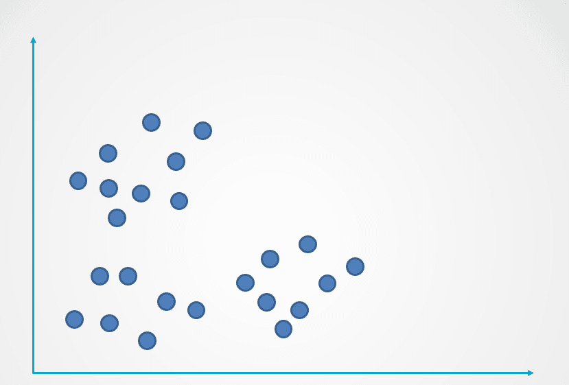
Image by author
Step 1: The image above consists of unlabeled observations that have not been grouped. Initially, each observation will be assigned to a cluster at random. A centroid will then be computed for each cluster.
These are represented with the “+” symbol in the diagram below:
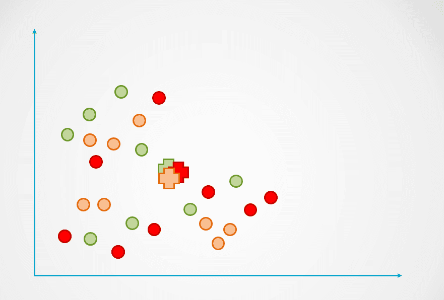
Image by author
Step 2: Next, the distance of each data point to the centroid is measured, and each point is assigned to the nearest centroid:
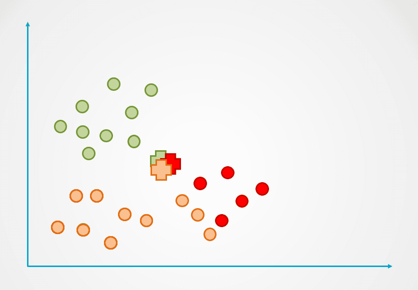
Image by author
Step 3: The centroid of the new cluster is then recalculated, and data points will be reassigned accordingly.
Step 4: This process is repeated until data points are no longer being reassigned:
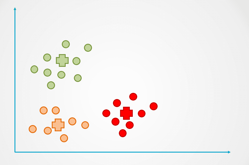
Image by author
Observe that three clusters were created in the example above. The number of clusters is referred to as “k” in the K-Means clustering algorithm, and this has to be determined by us.
There are a few different ways to select “k” in K-Means, the most popular of which is the elbow method. This technique consists of plotting the error for a different number of clusters on a graph and choosing the inflection point of the curve as “k.”
Learn more in our K-Means clustering in Python tutorial to discover the elbow method and the inner workings of K-Means clustering.
from sklearn.cluster import KMeans
kmeans = KMeans(n_clusters = 3, init='k-means++')
The n_clusters argument indicates the number of clusters “k” that you need to define when building the algorithm.
If you managed to follow along with this entire article, congratulations! You now know about some of the most popular supervised and unsupervised machine learning models and algorithms and how they can be applied to solve a variety of predictive modeling problems.
To become a data scientist, you need to understand how different types of machine learning models work to apply them to solve a problem. For instance, if you’d like to build a model that is interpretable and has low computation time, it might make sense to create a decision tree. If your aim is to create a model that generalizes well, however, then you can choose to build a random forest algorithm instead.
It is also important to understand how to evaluate machine learning models. A “good” model is subjective and highly dependent on your use case. In classification problems, for instance, high accuracy alone isn’t indicative of a good model. As a data scientist, you need to review metrics like precision, recall, and F1-Score to get a better idea of how well your model is performing.
If you would like to gain a deeper understanding of machine learning models than the concepts covered in this article, take the Machine Learning Scientist with Python course. This career track will teach you the theory behind how machine learning models operate and how they can be implemented in Python. You will also learn data preparation techniques such as normalization, decorrelation, and feature selection in the course.
Machine Learning Courses
Course
Course
Course
blog
Matt Crabtree
14 min
blog
Zoumana Keita
14 min
blog
Kurtis Pykes
12 min
blog
Moez Ali
15 min
blog
Moez Ali
8 min
cheat-sheet
Richie Cotton