Lyric Analysis: Predictive Analytics using Machine Learning with R

If you need an intro to machine learning, take DataCamp's Introduction to Machine Learning course and check out the Introduction to Machine Learning in Python tutorial.

Use a variety of machine learning (ML) classification algorithms to build models step-by-step that predict the genre of a song and whether it will be successful on the Billboard charts - based entirely on lyrics!

This is Part Three of a three-part tutorial series in which you will continue to use R to perform a variety of analytic tasks on a case study of musical lyrics by the legendary artist Prince, as well as other artists and authors. The three tutorials cover the following:

• Part One: Lyric Analysis with NLP & Machine Learning with R
• Part Two-A: Tidy Sentiment Analysis in R
• Part Two-B: Machine Learning and NLP using R - Topic Modeling and Music Classification
• Part Three: Lyric Analysis: Predictive Analytics using Machine Learning with R

Introduction

As a Data Scientist, you will need to understand both supervised and unsupervised learning. This tutorial explains and provides a musical use case for a form of supervised learning, specifically classification, that is based on the lyrics of a variety of artists (and a couple of book authors). You will learn how to build models to classify songs into their associated genre and to investigate the possibility of using lyrics to determine commercial success.

Goals

Have you ever used a music streaming and automated recommendation internet radio service like Pandora, iHeart Radio, Spotify, etc? If you have set up a hard rock station, you probably don't expect to hear a country song about cowboy boots and small towns. Typical music recommendation systems focus on sound qualities while lyrical analysis is just now appearing in research papers. With the techniques in this tutorial, you can utilize cutting edge methods being researched by scientists today to come up with ideas to advance this burgeoning field.

Prerequisites

This tutorial assumes a basic understanding of text mining using tidytext. It is an intermediate introduction to machine learning techniques using several popular classification algorithms. It is recommended that you have substantial experience with R programming, preferably with some knowledge of machine learning and want to learn more about its application and implementation through the hands-on use cases. Each algorithm is only briefly explained, but links are always provided for more in-depth analysis.

Throughout this article, you will be using a framework for machine learning experiments in R called mlr. Although this tutorial is not on mlr, you will utilize it extensively as a type of interface to the machine learning process. The goal is to use it to simplify the explanation of the various steps to building a model using different algorithms. I highly recommend this comprehensive tutorial on the package.

Considerations

There are many, many components to ML and you will only scratch the surface in this tutorial. Unlike Parts One and Two of this series, the narration may leave you with more questions than answers. You will get the most out of the experience if you plug along with your own data and code, and research the different algorithms at your own pace.

Steps

Here is a high-level outline of the steps to build your models:

Section One: Learn how to predict genre based on lyrical features.

• Read in lyrics/text of 10 different artists/authors (two per genre for five genres)
• Create training and test tidy dataframes
• Perform feature engineering to create predictors for your models
• Identify the algorithms to use for classification
• Train your models and benchmark the best options
• Pick a model and tune
• Test your model on a new dataset

Section Two: Use the lyrics of the iconic artist, Prince, to develop models to predict song success.

Preparation

You'll want to check out the previous tutorials to truly understand the data and its nuances. Keep in mind that mining and predictive analytics on lyrics is very complicated compared to non-fiction in that the context, meaning, and subtle messages are often hidden beneath the creative nuances implied by the songwriter. As with Part Two-B on topic modeling, you will continue to work with artists of different genres and with the contents of two books on machine learning (with a genre of data science - for the purpose of introducing another form of text).

Libraries and Functions

Start by loading the libraries and then take a look at the overall structure of the data.

 library(tidyverse) #tidyr, #dplyr, #magrittr, #ggplot2
library(tidytext) #unnesting text into single words
library(mlr) #machine learning framework for R
library(kableExtra) #create attractive tables
library(circlize) #cool circle plots
library(jpeg) #read in jpg files for the circle plots

#define some colors to use throughout
my_colors <- c("#E69F00", "#56B4E9", "#009E73", "#CC79A7", "#D55E00", "#D65E00")

#customize the text tables for consistency using HTML formatting
my_kable_styling <- function(dat, caption) {
  kable(dat, "html", escape = FALSE, caption = caption) %>%
  kable_styling(bootstrap_options = c( "condensed", "bordered"),
                full_width = FALSE)
}

Just for Fun

As with the previous tutorials, the code for this circle plot below can look complicated, but I can never resist a cool graphic. This shows you an album/book cover for each of the artists/authors in your data. This covers the test and training datasets. For more details on the circlize package, check out this book by Zuguang Gu.

 #read in the list of jpg files of album/book covers
files = list.files("jpg\\", full.names = TRUE)

#clean up the file names so we can use them in the diagram
removeSpecialChars <- function(x) gsub("[^a-zA-Z]", " ", x)
names <- lapply(files, removeSpecialChars)
names <- gsub("jpg","", names )

#check out the circlize package for details!
circos.clear() #very important!
circos.par("points.overflow.warning" = FALSE)
circos.initialize(names, xlim = c(0, 2))
circos.track(ylim = c(0, 1), panel.fun = function(x, y) {
  image = as.raster(readJPEG(files[CELL_META$sector.numeric.index]))
  circos.text(CELL_META$xcenter, CELL_META$cell.ylim[1] - uy(1.5, "mm"),
              CELL_META$sector.index,
              CELL_META$sector.index, facing = "clockwise", niceFacing = TRUE,
              adj = c(1, 0.5), cex = 0.9)
  circos.raster(image, CELL_META$xcenter, CELL_META$ycenter, width = "1.5cm",
        facing = "downward")
}, bg.border = 1, track.height = .4)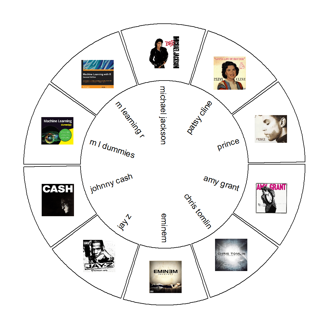

Get the Data

In order to focus on modeling, I performed data conditioning outside of this tutorial and have provided you with all the data you need for analysis. Here is a summary of the pre-processing:

• scraped the web for lyrics of eight artists
• used the pdf_text() function from the pdftools package to collect the content of two books (each page represents a distinct document)
• cleaned all the data by removing undesirable characters and converted to lower case as described in Part One
• combined and balanced the data such that each writer (source) has the same number of songs/documents

Below you will read in the training and test data which are already split for you to load separately. Then use unnest() from tidytext to create the tidy version with one word per record.

 five_sources_data <- read.csv("five_sources_data_balanced.csv", stringsAsFactors = FALSE)

five_sources_tidy <- five_sources_data %>%
  unnest_tokens(word, text) %>%
  anti_join(stop_words)

five_sources_data_test <- read.csv("five_sources_data_test.csv", stringsAsFactors = FALSE)

five_sources_test_tidy <- five_sources_data_test %>%
  unnest_tokens(word, text) %>%
  anti_join(stop_words)

#very small file that has a couple of words that help to identify certain genres
explicit_words <- read.csv("explicit_words.csv", stringsAsFactors = FALSE)

Examine the Data

Now that you have train and test data loaded and tidied, you can see how many songs exist per artist/author. Since the dataset has songs and book pages, I'll refer to them each as a document. The features that you will create are based on documents and their associated metadata, so it's important to understand this concept. Also, because there are artists and authors, I will refer to them as the source of each document.

 five_sources_data %>%
  group_by(genre, source) %>%
  summarise(doc_count = n()) %>%
  my_kable_styling("Training Dataset")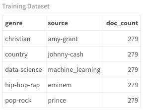

 five_sources_data_test %>%
  group_by(genre, source) %>%
  summarise(doc_count = n()) %>%
  my_kable_styling("Test Dataset")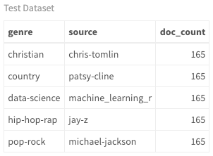

Although you can see the genre, source, and the number of documents, the following chord diagram is a better way to view these relationships. Throughout the tutorial, you can see the progression of how these relationships change with your new models. Currently there is a one-to-one relationship between source and genre because the artists are classified this way; however, cross-over artists are very common, and you'll see evidence of that when you look at the later versions of this diagram.

 #get SONG count per genre/source. Order determines top or bottom.
genre_chart <-  five_sources_data %>%
  count(genre, source)  

circos.clear() #very important! Reset the circular layout parameters
#assign chord colors
grid.col = c("christian" = my_colors[1], "pop-rock" = my_colors[2],
             "hip-hop-rap" = my_colors[3], "data-science" = my_colors[4],
             "country" = my_colors[5],
             "amy-grant" = "grey", "eminem" = "grey",
             "johnny-cash" = "grey", "machine_learning" = "grey",
             "prince" = "grey")
# set the global parameters for the circular layout. Specifically the gap size
circos.par(gap.after = c(rep(5, length(unique(genre_chart[[1]])) - 1), 15,
                         rep(5, length(unique(genre_chart[[2]])) - 1), 15))

chordDiagram(genre_chart, grid.col = grid.col, transparency = .2)
title("Relationship Between Genre and Source")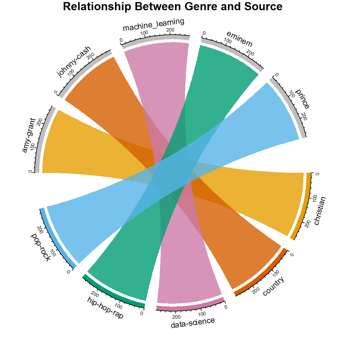

Think about what this diagram would look like if there was not a one-to-one relationship. If you were to predict genre based only on lyrics, what do you think it would happen?

Predict Genre

If all you had to work with in order to classify a song was lyrics, how would you generate predictor variables? First think about the song and what makes one different from another, lyrically. A common theme in all music is repetition. Do some genres use repetition more than others? What about word length? Do some use larger or smaller words more often? What other factors can you think of to describe lyrics? If you get these counts per song, you have your first set of predictors!

Note that all of the variables listed above are quantitative features, (counts, lengths, etc.) based on words per song. But what about individual words specific to genres? In previous tutorials, you worked on sentiment analysis and topic modeling. These activities were focused on words that were specific to certain artists or genres. So if you take that a step further, you can create some of the most important predictive components that are based on content (or context). This is the creative step that is specific to text analytics and results in critical predictors for your models.

Feature Engineering

First, you want to get the most common (frequently used) words per genre. This was done in the Part One tutorial. Start by getting the total number of words per genre. Then group by words per genre and get a count of how often each word is used. Now select the top n most frequent words defined by the number_of_words variable. This is the tricky part: how many words should you choose? If you don't select enough, you will not optimize the model, but if you select too many, you overfit and distort the results. This is relatively complicated to describe, but the real solution is trial and error. I came up with a total of 5500 as the most optimal number of words. Play around with this value and see how it impacts your outcome. You may find a better result! If this step is not completely clear yet, stay with me and it will begin to make more sense.

Many words are very common to more than one genre (such as time, life, etc.) and I have removed these words with the multi_genre variable below. This makes for a cleaner list of distinct words that create a better distinction between the sources.

 #play with this number until you get the best results for your model.
number_of_words = 5500

top_words_per_genre <- five_sources_tidy %>%
  group_by(genre) %>%
  mutate(genre_word_count = n()) %>%
  group_by(genre, word) %>%
  #note that the percentage is also collected, when really you
  #could have just used the count, but it's good practice to use a %
  mutate(word_count = n(),
         word_pct = word_count / genre_word_count * 100) %>%
  select(word, genre, genre_word_count, word_count, word_pct) %>%
  distinct() %>%
  ungroup() %>%
  arrange(desc(word_pct)) %>%
  top_n(number_of_words) %>%
  select(genre, word, word_pct)

#remove words that are in more than one genre
top_words <- top_words_per_genre %>%
  ungroup() %>%
  group_by(word) %>%
  mutate(multi_genre = n()) %>%
  filter(multi_genre < 2) %>%
  select(genre, top_word = word)

#create lists of the top words per genre
book_words <- lapply(top_words[top_words$genre == "data-science",], as.character)
country_words <- lapply(top_words[top_words$genre == "country",], as.character)
hip_hop_words <- lapply(top_words[top_words$genre == "hip-hop-rap",], as.character)
pop_rock_words <- lapply(top_words[top_words$genre == "pop-rock",], as.character)
christian_words <- lapply(top_words[top_words$genre == "christian",], as.character)

Now use the genre-specific words as features in your dataset. Since you'll be creating features for multiple datasets, create a function so that you only have to write it out once. In this function, you see references to lexical diversity and density. Check out Part One for an explanation of these concepts.

Think about each feature below and how it could vary according to the genre. Rather than explaining each feature, I will focus on the machine learning steps that follow, so take a minute to review the code and understand what it's doing. And don't forget the critical genre specific predictors. As an example, country_word_count is merely a count of the top country words that appear in each song. Notice that I have assigned more weight to explicit and book words (see the 10 and 20 used in the sum() function). I did this because they are very distinctive and help to classify documents. Again, this was a trial and error process!

 
features_func_genre <- function(data) {
  features <- data %>%
  group_by(document) %>%
  mutate(word_frequency = n(),
         lexical_diversity = n_distinct(word),
         lexical_density = lexical_diversity/word_frequency,
         repetition = word_frequency/lexical_diversity,
         document_avg_word_length = mean(nchar(word)),
         title_word_count = lengths(gregexpr("[A-z]\\W+",
                                             document)) + 1L,
         title_length = nchar(document),
         large_word_count =
           sum(ifelse((nchar(word) > 7), 1, 0)),
         small_word_count =
           sum(ifelse((nchar(word) < 3), 1, 0)),
         #assign more weight to these words using "10" below
         explicit_word_count =
          sum(ifelse(word %in% explicit_words$explicit_word,10,0)),
         #assign more weight to these words using "20" below
         book_word_count =
           sum(ifelse(word %in% book_words$top_word,20,0)),
         christian_word_count =
           sum(ifelse(word %in% christian_words$top_word,1,0)),
         country_word_count =
           sum(ifelse(word %in% country_words$top_word,1,0)),
         hip_hop_word_count =
           sum(ifelse(word %in% hip_hop_words$top_word,1,0)),
         pop_rock_word_count =
           sum(ifelse(word %in% pop_rock_words$top_word,1,0))
         ) %>%
  select(-word) %>%
  distinct() %>% #to obtain one record per document
  ungroup()

features$genre <- as.factor(features$genre)
return(features)
}

Now call your features() function for your training and test datasets.

 train <- features_func_genre(five_sources_tidy)
test  <- features_func_genre(five_sources_test_tidy)

Machine Learning Process

If you haven't used the mlr package before, it's ok. You'll take it step by step and see that it's actually a straight forward process. Again, I highly recommend reviewing this tutorial as it is the most comprehensive documentation you can find on this package. You could also visit mlr.org as well.

mlr (Machine Learning for R), is a framework that includes all of the frequently used machine learning algorithms. Rather than explaining the theory behind each algorithm, I will instead focus on their implementation. By the end of this tutorial, you will have utilized many classification tools, and you will get the most out of it if you practice alongside the code presented here.

Once you've done your feature engineering, the ML process is simple: create a task, make a learner, train it, test it. Here are the steps you will take:

• Create the classifier task: declare the datasets and outcome (target) variable
• Normalize the data: pre-processing (scale and center)
• Create a list of learners: choose the learning algorithm(s)
• Choose a resampling method: choose a method to assess performance using a validation set during training
• Select the measures: create a list of measures such as accuracy or error rate
• Perform training/benchmarking: compare the results of the models based on the tasks and learners
• Tune the best model: choose the best performing learner and tune the hyperparameters
• Test on new data: run your model against data it has never seen before

The Classifier Task

A task is merely the dataset on which a learner learns. Since this is a classification problem, you will create a classification task by using makeClassifTask(). You need to specify your classification outcome variable, genre, by passing it as the target argument.

I have created three tasks below, each with a different purpose. Test and train are obvious, but there is also a dataset that uses only the basic quantitative features consisting of document summaries and counts. This task, task_train_subset is created without the genre word count features (i.e., country_word_count, pop_rock_word_count, etc.) to illustrate the importance of these contextual predictors in the final model. So using the dataset train[3:13] removes these variables. Also, you always want to remove the text columns when creating the classifier task. In this case, they are in positions one and two in the dataframe.

 #create classification tasks to use for modeling

#this dataset does not include genre specific words
task_train_subset <- makeClassifTask(id = "Five Sources Feature Subset",
                                     data = train[3:13], target = "genre")

#create the training dataset task
task_train <- makeClassifTask(id = "Five Sources",
                              data = train[-c(1:2)], target = "genre")

#create the testing dataset task
task_test <- makeClassifTask(id = "New Data Test",
                             data = test[-c(1:2)], target = "genre")

Normalize Data

Normalizing data is a topic that requires a little investigation, is not always necessary, and depends on the dataset; however, in this case, it is beneficial. It is simply a method of scaling your data such that all the values are normalized between values of zero and one (or whatever values you pass). If some variables are much larger in value and are on a different scale than the others, they will throw off your model by giving more weight to those variables. Normalization takes care of this problem. Here is a good thread on the topic. It's definitely worth further investigation as it's an important step in pre-processing. mlr provides a simple function called normalizeFeatures() for this step.

 
#scale and center the training and test datasets
task_train_subset <- normalizeFeatures(task_train_subset, method = "standardize",
  cols = NULL, range = c(0, 1), on.constant = "quiet")

task_train <- normalizeFeatures(task_train, method = "standardize",
  cols = NULL, range = c(0, 1), on.constant = "quiet")

task_test <- normalizeFeatures(task_test, method = "standardize",
  cols = NULL, range = c(0, 1), on.constant = "quiet")

Create a List of Learners

A learner in mlr is generated by calling makeLearner(). In the constructor, you need to specify which learning method you want to use. You can obtain a list of possible classification algorithms by calling listLearners("classif")[c("class","package")]. This shows you the algorithms you have to choose from as well as their dependent packages (which you may need to install separately).

For this exercise, I've chosen a list that can handle more than two classes and will give you a wide range of techniques, from decision trees to random forests, support vector machines, gradient boosting, and neural networks. There are many learners from which to choose (currently there are over 80 classification learners in mlr), and I encourage you to play around with them!

 #create a list of learners using algorithms you'd like to try out
lrns = list(
makeLearner("classif.randomForest", id = "Random Forest", predict.type = "prob"),
makeLearner("classif.rpart", id = "RPART", predict.type = "prob"),
makeLearner("classif.xgboost", id = "xgBoost", predict.type = "prob"),
makeLearner("classif.kknn", id = "KNN"),
makeLearner("classif.lda", id = "LDA"),
makeLearner("classif.ksvm", id = "SVM"),
makeLearner("classif.PART", id = "PART"),
makeLearner("classif.naiveBayes", id = "Naive Bayes"),
makeLearner("classif.nnet", id = "Neural Net", predict.type = "prob")
)

Resampling

Resampling is an essential tool in machine learning and deserves an entirely separate tutorial. For now, a basic understanding of it can help you through this step. It involves repeatedly drawing samples from a training set and refitting a model on each sample. This may allow you to obtain information not available from fitting the model only once with the original training data.

There are several methods of resampling, but here you will use what's called k-fold cross validation indicated by the "CV" in the call to makeResampleDesc() which returns a resample description object (rdesc). This approach randomly divides the dataset into k groups (folds) of equal size. The first fold is used as a validation set, and the remaining folds are used for training. This is repeated k times on each of the folds. The error rate is captured for each iteration and averaged at the end.

This may sound Greek if it's the first time you've dealt with resampling, but it is an essential first step to get familiar with the concept! You'll be using 10-fold cross-validation in your example below. "For classification, it is usually desirable to have the same proportion of the classes in each fold." (Source) Use stratify = TRUE to ensure this happens.

For more information on resampling within mlr, check out this article.

 # n-fold cross-validation
#use stratify for categorical outcome variables
rdesc = makeResampleDesc("CV", iters = 10, stratify = TRUE)

Performance Measures

The typical objective of classification is to obtain a high prediction accuracy and minimize the number of errors. In this sense, all types of misclassification errors are considered with equal weight. However, in many applications, different kinds of errors have more impact than others. For example, if you were classifying whether a patient has a disease or not, a misclassification that doesn't identify disease when it is actually there could be life-threatening. Different performance measures address these nuances. For lyric analysis however, you will mostly look at the basic measures of accuracy and error. Just remember that accuracy and error rate are not always the best choices to evaluate the robustness of a model. This is an important topic that also deserves more discussion outside of this tutorial.

Accuracy is the number of correct predictions from all predictions made. To examine the misclassifications by your model, you will also look at a confusion matrix to see how things were classified (predicted vs. actual). More on that in just a minute. Right now, just set up a list of measures of interest. I've added three measures here, but you'll just look at acc. This link will give you more information and explanation of performance measures.

 #let the benchmark function know which measures to obtain
#accuracy, time to train
meas = list(acc, timetrain)

Train Models / Benchmark

In mlr, you can conduct a benchmark experiment in which different algorithms (learning methods) are applied to your dataset. This allows you to compare algorithms according to the specific measures of interest (i.e., accuracy). You will run benchmark() to train your model and generate a BenchmarkResult object from which you can access the models and results.

Feature Subset

Finally, it's time to build a model. Start with the task you created that does not include the genre-specific word counts. Pass to benchmark your list of learners, the subset task, the resampling strategy (rdesc), and the list of measures you would like to see.

 #it would be best to loop through this multiple times to get better results
#so consider adding a for loop here!
set.seed(123)
bmr <- benchmark(lrns, task_train_subset, rdesc, meas, show.info = FALSE)

#I'm just accessing an aggregated result directly so you can see
#the object structure and so I can use the result in markdown narrative
rf_perf <- round(bmr$results$`Five Sources Feature Subset`$`Random Forest`$aggr[[1]],2) * 100

## [1] "BenchmarkResult"

class(bmr)
bmr

##                       task.id    learner.id acc.test.mean
## 1 Five Sources Feature Subset Random Forest     0.7282895
## 2 Five Sources Feature Subset         RPART     0.6516754
## 3 Five Sources Feature Subset       xgBoost     0.6871616
## 4 Five Sources Feature Subset           KNN     0.6676070
## 5 Five Sources Feature Subset           LDA     0.6632281
## 6 Five Sources Feature Subset           SVM     0.6965042
## 7 Five Sources Feature Subset          PART     0.6561634
## 8 Five Sources Feature Subset   Naive Bayes     0.6184923
## 9 Five Sources Feature Subset    Neural Net     0.7073271
##   timetrain.test.mean
## 1               0.892
## 2               0.013
## 3               0.062
## 4               0.000
## 5               0.007
## 6               0.222
## 7               0.218
## 8               0.012
## 9               0.252

If you look at the BenchmarkResult object, you can see the acc.test.mean for each of the algorithms you passed. Notice this specifically refers to test. This is the average accuracy across all samples for the validation datasets used in cross-validation when you trained the model. This is not the same as the test dataset that you'll use later on. This is another one of those topics that deserves a good deal of explanation, but again just keep in mind there is a series of validation datasets that are held out during cross-validation, and a test dataset that you'll use after you decide on an algorithm and tune the model.

In this benchmark experiment, you can see that Random Forest performs the best at r rf_perf percent (and took the longest to train). Keeping that value in mind, rerun this experiment on the full feature set.

Full Feature Set

This time pass the task that includes the genre-specific word count per document. This adds features that indicate whether a song has more country words, or pop-rock words, etc. Remember, using your labeled dataset, you selected the most common hip-hop words and put them in a list called hip_hop_words. This has words like thug, crib, and drug. The country word list has things like lonesome, coal, drunken, and cattle. You get the idea.

mlr provides several different methods for accessing benchmark results. I'll use just a few, but to get comfortable with the benchmark object, I recommend using the getBMR* getter functions. If you call str() on your benchMark object, you will be waiting for quite a while for it to return the details!

Before looking in detail at the full feature set, take a second to benchmark multiple tasks and compare the full feature set to the feature subset above using the plotBMRSummary() getter function. Do this by creating a list of tasks to pass to benchmark().

 #always set.seed to make sure you can replicate your results
set.seed(123)
task_list <- list(task_train, task_train_subset)
bmr_multi_task <- benchmark(lrns, task_list, rdesc, meas, show.info = FALSE)

plotBMRSummary(bmr_multi_task)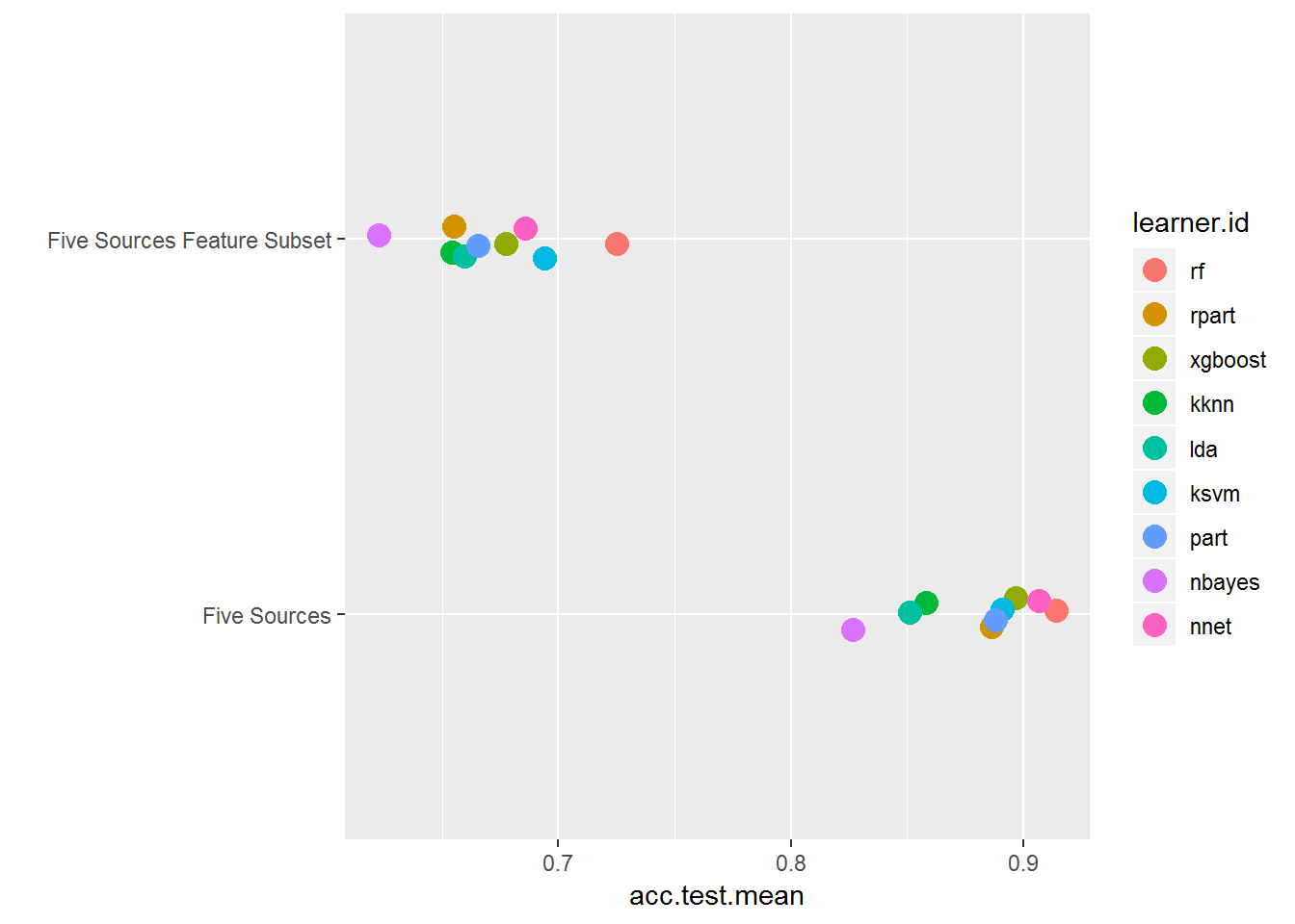

Here you can see the acc.test.mean of the training subset without the genre-specific word counts per document is lower than the full feature dataset. This indicates that these features make a huge difference! Performing this little creative step is something you will only see in machine learning using text. It's good to have this in your back pocket for projects of your own.

Although you could access just the training results from bmr_multi_task, go ahead and benchmark again with just the training task and then take a closer look at the results using getBMRAggrPerformances() and plotBMRBoxplots().

 set.seed(123)
bmr = benchmark(lrns, task_train, rdesc, meas, show.info = FALSE)

plotBMRSummary(bmr)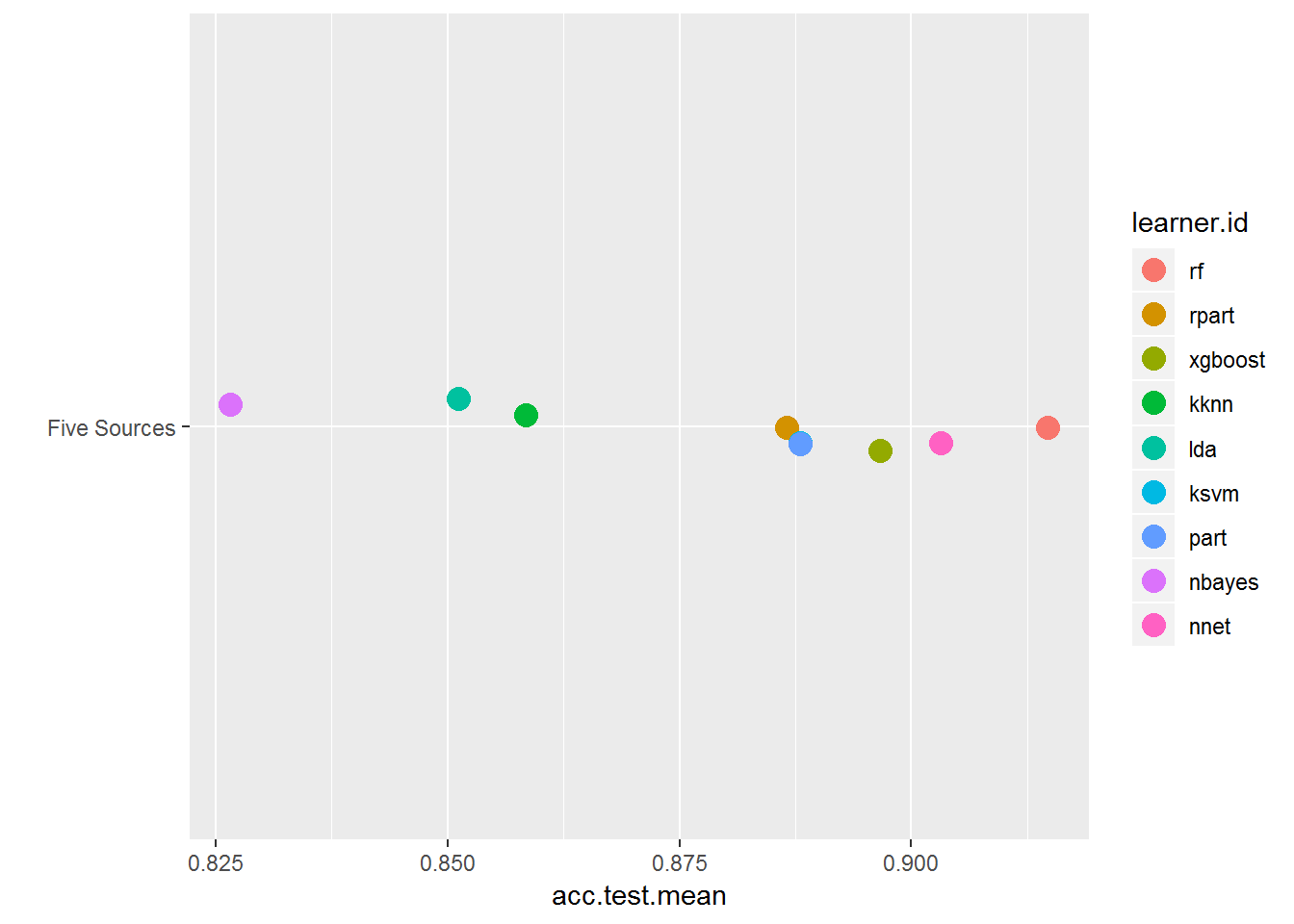

This just allows you to zoom in on the results of the fully featured dataset results. Now you can more clearly see the discrepancy between algorithms and how random forest outperforms the others.

 plotBMRBoxplots(bmr, measure = acc, style = "violin",
                pretty.names = FALSE) +
  aes(color = learner.id) +
  ylab("Accuracy") +
  theme(strip.text.x = element_text(size = 8))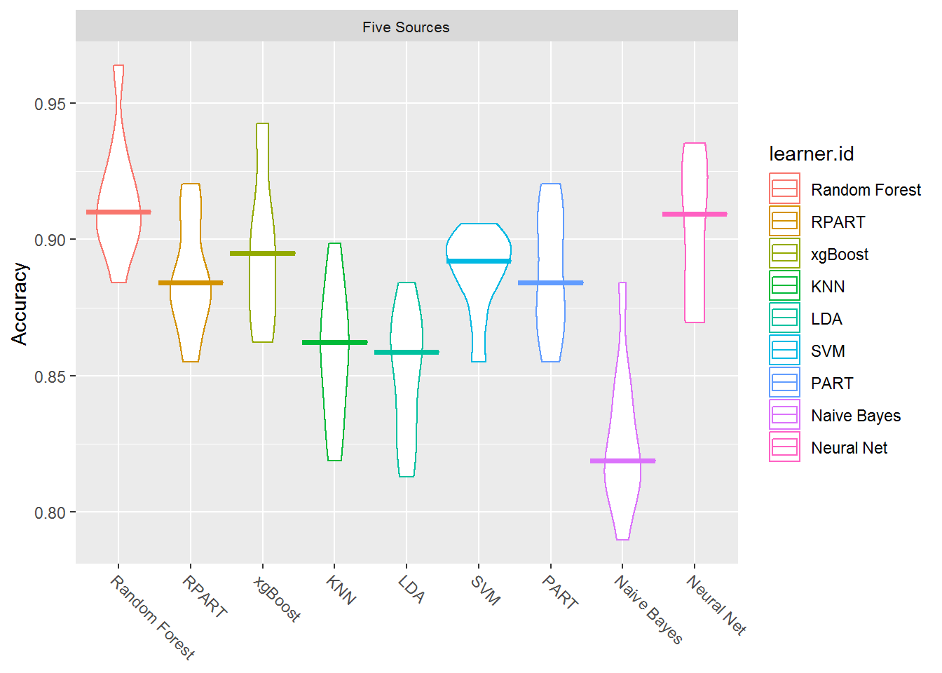

These boxplots show you the results for each method across several iterations performed by benchmarking.

 performances <- getBMRAggrPerformances(bmr, as.df = TRUE) %>%
  select(ModelType = learner.id, Accuracy = acc.test.mean) %>%
  mutate(Accuracy = round(Accuracy, 4)) %>%
  arrange(desc(Accuracy))

#just for use in markdown narrative
first_three <- round(performances$Accuracy[1:3],2) * 100

performances %>%
  my_kable_styling("Validation Set Model Comparison")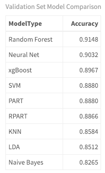

Here you can see the accuracy is highest for Random Forest, Neural Net, and xgBoost with accuracies of r first_three percentages, respectively. So what really happened with the model? How were these documents/songs actually classified? What were the most difficult genres to classify based on lyrics? To get more insight, look at the confusion matrix of the predictions. In this matrix, the number of correctly classified documents appear on the diagonal. Misclassified documents are on the off-diagonal. Error observation counts are in the margins. The columns represent the predicted values, and the rows represent the true values. Use getBMRPredictions() to access the training/validation set predictions. Then look at the result of the confusion matrix of the Random Forest model which you can access using the Five Sources id you labeled earlier as your training task. (Note that you could do this for any of the models in the benchmark results.)

 predictions <- getBMRPredictions(bmr)

calculateConfusionMatrix(predictions$`Five Sources`$`Random Forest`)$result  %>%
  my_kable_styling("Random Forest Confusion Matrix: Rows are True, Columns are Predictions")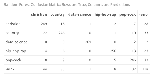

You finally have some insight into your model! As you may expect, with only one misclassification, it is relatively easy to distinguish data science documents from song lyrics using the textual metadata features you engineered. In addition, hip-hop-rap is very distinctive from other musical genres with only eight misclassifications. However, although performance is quite impressive, there is less distinction between country, Christian and pop-rock musical lyrics.

The point of this tutorial is not only to get exposure to predictive machine learning techniques but also to perform lyric analysis as a continuation of previous tutorials in this series. So think about what these results mean. If you were developing a recommendation system that is supplemented with lyrical insights, what considerations should you make? Is there a chance that your system may recommend a hip hop artist with explicit lyrics for a Christian music listener or a country music fan?

Remember the chord diagram at the beginning of the tutorial? Retake a look at it, this time with predictions rather than true labels.

 train$id <- seq_len(nrow(train))
df <- predictions$`Five Sources`$`Random Forest`$data

chart <- train %>%
  inner_join(predictions$`Five Sources`$`Random Forest`$data) %>%
  group_by(source, response) %>%
  summarise(n())

circos.clear() #very important! Reset the circular layout parameters
#assign chord colors
grid.col = c("christian" = my_colors[1], "pop-rock" = my_colors[2],
             "hip-hop-rap" = my_colors[3], "data-science" = my_colors[4],
             "country" = my_colors[5],
             "amy-grant" = my_colors[1], "prince" = my_colors[2],
             "eminem" = my_colors[3], "machine_learning" = my_colors[4],
             "johnny-cash" = my_colors[5])

# set the global parameters for the circular layout. Specifically the gap size
circos.par(gap.after = c(rep(5, length(unique(chart[[1]])) - 1), 15,
                         rep(5, length(unique(chart[[2]])) - 1), 15))

chordDiagram(chart, grid.col = grid.col, transparency = .2)
title("Predicted Relationship Between Genre and Source - Train")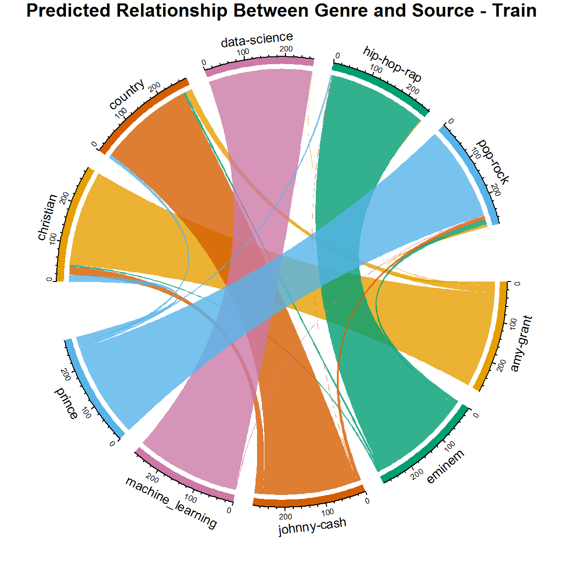

Pretty cool. Now you can see how well you did on the training data. Once again the results are impressive. The smaller lines represent the misclassifications. But here is probably the most important concept you can get out of this tutorial: even though this is the validation set accuracy results, this is still based on a labeled training dataset! If you aren't careful, you may overfit your model and introduce high variance. High variance means that your learning algorithm varies a lot depending on the data that you give it. This could mean your algorithm may not be robust to noise that can be introduced with new data it has not seen before. You will run a true test of the model in just a bit when you feed it brand new data.

Before you test new data, you'll want to pick one of the models and tune it. You will do this by adjusting its hyperparameters. This is just a fancy word meaning to configure the parameters of your model to improve its performance. If you've visited Kaggle recently, you have noticed a trendy algorithm called extreme gradient boosting that is dominating the competitions. Even though it was not the top performing model in our benchmark, I'm still going to choose it to tune and run on our test dataset. If you're new to this type of algorithm, tuning will probably be the hard part. Given the scope of this tutorial, I cannot go into the concepts behind extreme gradient boosting or even the hyperparameters, but the code below will give you a starting point. I highly recommend reviewing the concept of gradient boosting before getting too deep into tuning the parameters. This link provides a great article by Prince Grover to get you started. As he describes it, here is a general summary of classic gradient boosting:

First model data with simple models and analyze data for errors. These errors signify data points that are difficult to fit by a simple model. Then for later models, particularly focus on those hard to fit data to get them right. In the end, combine all the predictors by giving some weights to each predictor.

(Just a side note: the maxit value of 150 in makeTuneControlRandom() below takes quite some time to run. You may want to start out with something much smaller to get started.)

Tune the model - xgBoost

 #experiment here!! this is where you can really improve your model
xgb_params <- makeParamSet(
  makeDiscreteParam("booster",values = c("gbtree")),
  makeIntegerParam("nrounds",lower=10,upper=20),
  makeIntegerParam("max_depth",lower = 4,upper = 6),
  makeNumericParam("min_child_weight",lower = 1L,upper = 10L),
  makeNumericParam("subsample",lower = 0.5,upper = 1),
  makeNumericParam("colsample_bytree",lower = 0.5,upper = 1),
  makeNumericParam("eta",lower = .01, upper = .2)
)
control <- makeTuneControlRandom(maxit = 150L)

xglearn <- makeLearner("classif.xgboost", predict.type = "prob", id="tuned xgboost")

library(parallelMap)
parallelStartSocket(2)
set.seed(123)
tuned_params <- tuneParams(
  learner = xglearn,
  task = task_train,
  resampling = rdesc,
  par.set = xgb_params,
  control = control,
  measures = acc,
  show.info = TRUE
)

xgb_tuned_learner <- setHyperPars(
  learner = xglearn,
  par.vals = tuned_params$x
)

tuned_params$x
 

## $booster
## [1] "gbtree"
##
## $nrounds
## [1] 16
##
## $max_depth
## [1] 5
##
## $min_child_weight
## [1] 1.395328
##
## $subsample
## [1] 0.6397534
##
## $colsample_bytree
## [1] 0.7986664
##
## $eta
## [1] 0.1917797

You can examine the optimized parameters by looking at the output of tuneParams(). Now you want to create a new model using the tuned hyperparameters and then re-train on the training dataset.

lrns = list(makeLearner("classif.nnet", predict.type = "prob"),
            makeLearner("classif.PART", predict.type = "prob"),
            makeLearner("classif.randomForest", predict.type = "prob"),
            makeLearner("classif.xgboost", id="untunedxgboost" ,predict.type = "prob"),
            xgb_tuned_learner)

set.seed(123)
bmr = benchmark(lrns, task_train, rdesc, meas)
plotBMRBoxplots(bmr, measure = acc, style = "violin", pretty.names = FALSE) +
  aes(color = learner.id) +
  ylab("Accuracy") +
  theme(strip.text.x = element_text(size = 8))

 performances <- getBMRAggrPerformances(bmr, as.df = TRUE) %>%
  select(ModelType = learner.id, Accuracy = acc.test.mean) %>%
  mutate(Accuracy = round(Accuracy, 4)) %>%
  arrange(desc(Accuracy))

# #used in markdown
# first_three <- round(performances$Accuracy[1:3],2) * 100

performances %>%
  my_kable_styling("Validation Set Model Comparison")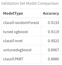

The tuned xgBoost model is only slightly higher than the untuned one and is still not as accurate as random forest. But how do they perform on the test data?

The Real Test: New Data

Now that you have your tuned model and benchmarks, you can call predict() for your top three models on the test dataset that has never been seen before. This includes five completely different sources as shown previously. Take a look at its performance and actual classifications.

 set.seed(12)
rf_model = train("classif.randomForest", task_train)
result_rf <- predict(rf_model, task_test)
performance(result_rf, measures = acc)

##       acc
## 0.6541262

set.seed(12)
nnet_model = train("classif.nnet", task_train)

## # weights:  68
## initial  value 2500.439406
## iter  10 value 876.420114
## iter  20 value 531.977942
## iter  30 value 412.756436
## iter  40 value 334.449379
## iter  50 value 304.202353
## iter  60 value 295.229853
## iter  70 value 286.347519
## iter  80 value 282.524065
## iter  90 value 280.438058
## iter 100 value 278.713625
## final  value 278.713625
## stopped after 100 iterations

result_nnet <- predict(nnet_model, task_test)
performance(result_nnet, measures = acc)

##      acc
## 0.631068

set.seed(12)
xgb_model = train(xgb_tuned_learner, task_train)
result_xgb <- predict(xgb_model, task_test)
test_perf <- performance(result_xgb, measures = acc)
test_perf

##       acc
## 0.6492718

These are pretty interesting results. Even though random forest had a higher accuracy on the training data than the tuned xgBoost, it was slightly less accurate on the test dataset. The test accuracy for neural net is much lower than on training as well. Neural nets can be very flexible models and as a result, can overfit the training set.

At an accuracy rate of r round(test_perf,2)*100% for tuned xgBoost, there was still a dramatic decrease in performance on the test data compared to training and tuning only made a slight improvement (using this minimal configuration!). This drop in accuracy between train and test is widespread and is precisely why you should test your model on new data.

Now, look at the actual classifications.

 calculateConfusionMatrix(result_xgb)$result %>%
  my_kable_styling("TEST: xgBoost Confusion Matrix: Rows are True, Columns are Predictions")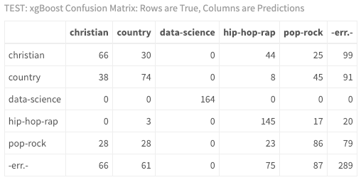

In looking at the confusion matrix, you can now see that it was much harder to classify this hip hop artist, Jay-Z. It's ok if you don't know the music, your results indicate that there may be a discrepancy between the artist used to train your model Eminem, and Jay-Z used in the test data. Ideally, you would have more data, more artists, more tuning, and you would run your model multiple times!!

However, think about what this could be telling you. Look at the chord diagram once again:

 test$id <- seq_len(nrow(test))

chart <- test %>%
  inner_join(result_xgb$data) %>%
  group_by(source, response) %>%
  summarise(n())

circos.clear() #very important! Reset the circular layout parameters
#assign chord colors
grid.col = c("christian" = my_colors[1], "pop-rock" = my_colors[2],
             "hip-hop-rap" = my_colors[3], "data-science" = my_colors[4],
             "country" = my_colors[5],
             "chris-tomlin" = my_colors[1], "michael-jackson" = my_colors[2],
             "jay-z" = my_colors[3], "machine_learning_r" = my_colors[4],
             "patsy-cline" = my_colors[5])

# set the global parameters for the circular layout. Specifically the gap size
circos.par(gap.after = c(rep(5, length(unique(chart[[1]])) - 1), 15,
                         rep(5, length(unique(chart[[2]])) - 1), 15))

chordDiagram(chart, grid.col = grid.col, transparency = .2)
title("Predicted Relationship Between Genre and Source - Test")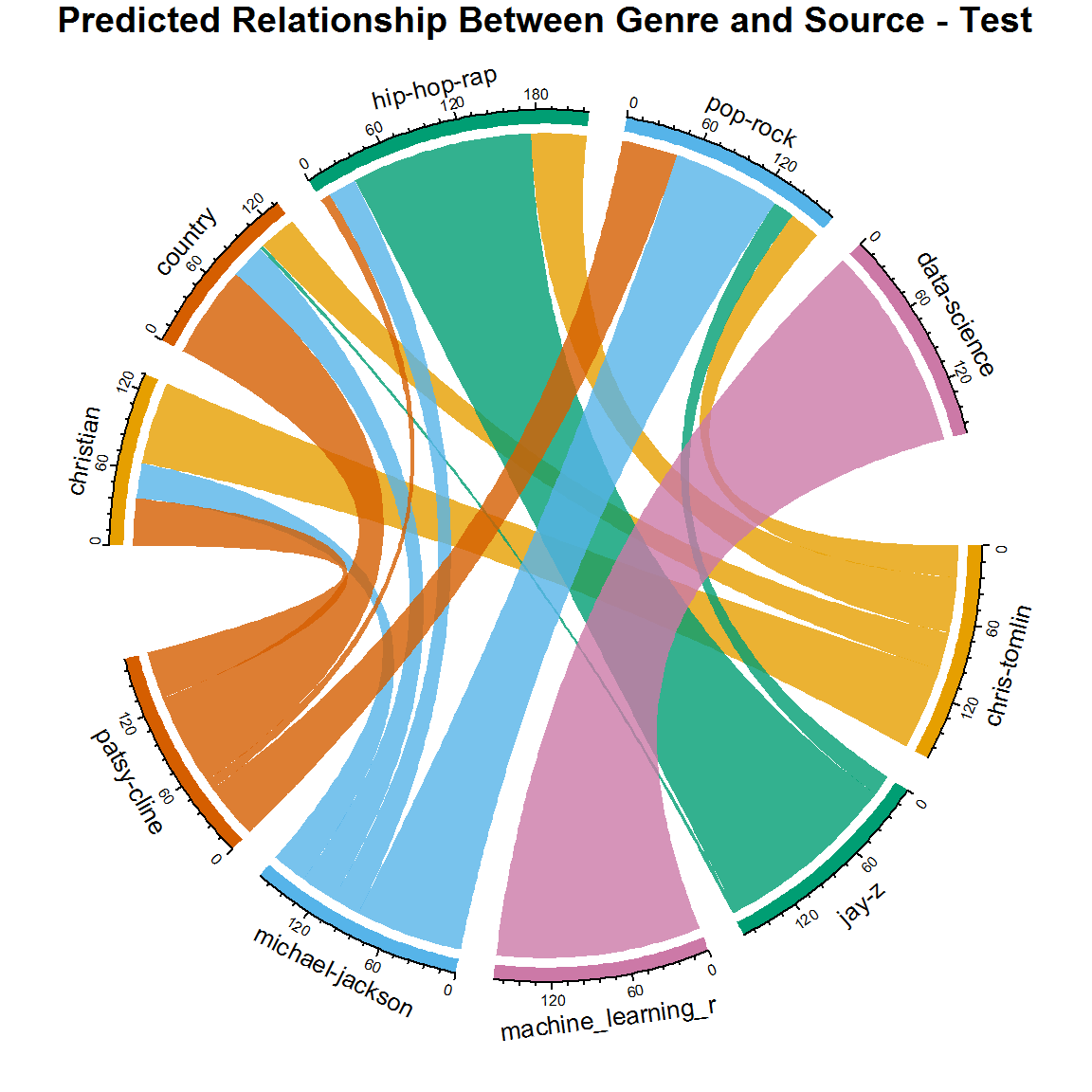

Is it wrong? Is it inaccurate? Is it insightful? I think you're getting a real glimpse into the world of music. Think about it: did Michael Jackson ever collaborate with rap artists? Did he ever sing about religious topics? Have country artists ever crossed over to pop-rock? Your new chord diagram actually gives a more realistic version of the lyrical classification than shown in the original dataset! There actually isn't a one-to-one relationship between artist, and genre in real life and that flexibility is built into your model.

Predict Chart Level

For the next part of the tutorial, you'll look at an idea that could be applied in marketing, sales, science, economics, etc., but here you will apply it to music. The success of a song is very subjective. The concept of commercial success is a little clearer as it can be defined by industry standards. The Billboard Charts (and many others) are example measures of such success. If you were to work for a recording label and trying to decide what artists to sign - or which signed artists to promote, wouldn't it be interesting if you could predict whether or not they will rank on the charts based on their lyrics using scientific methods? You would need a lot of current data and tons of metadata describing each song. Since your resources are limited here, just take what you have and test out the idea on Prince's lyrics with labeled chart data.

Get the Data

In previous tutorials, you created a dataset of Prince's songs where the majority of songs were uncharted. You'll be using a balanced set of lyrics with the same number of charted vs. uncharted songs. Here are the numbers:

 prince_charted_data <- read.csv("prince_data_balanced.csv", stringsAsFactors = FALSE)

prince_charted_data %>%
  count(charted) %>%
  my_kable_styling("Prince Data")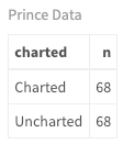

 prince_tidy <- prince_charted_data %>%
  unnest_tokens(word, lyrics) %>%
  anti_join(stop_words)

Feature Engineering

Using the same process as above, create the features using a two-step process. This time instead of counting words per genre in a song, you will count words per chart level. In other words, get the most frequently used words for songs that charted and most frequently used words for songs that did not chart and store them in lists. I chose to use 1000 words and seemed to get the best response with that number. Play around with your own values. Then when creating the song features, make sure to add these two features that count the number of words in each list per song (same process you used with genre above).

Notice again that I removed all words that appear in both the top charted and uncharted songs. I also added a few additional polynomial features where I squared the original inputs. This idea of improving a model not by tuning the algorithm, but by transforming the inputs, is fundamental to machine learning methods.

 number_of_words <- 1000

top_words_per_chart <- prince_tidy %>%
  group_by(charted) %>%
  mutate(chart_word_count = n()) %>%
  group_by(charted, word) %>%
  mutate(word_count = n(),
         word_pct = word_count / chart_word_count * 100) %>%
  select(word, charted, chart_word_count, word_count, word_pct) %>%
  distinct() %>%
  ungroup() %>%
  arrange(word_pct) %>%
  top_n(number_of_words) %>%
  select(charted, word, word_pct)

top_words <- top_words_per_chart %>%
  ungroup() %>%
  group_by(word) %>%
  mutate(multi_chart = n()) %>%
  filter(multi_chart < 2) %>%
  select(charted, top_word = word)

charted_words <- lapply(top_words[top_words$charted == "Charted",],
                        as.character)
uncharted_words <- lapply(top_words[top_words$charted == "Uncharted",],
                          as.character)


features_func_chart <- function(data, remove) {
  features <- data %>%
  group_by(song) %>%
  mutate(word_frequency = n(),
         lexical_diversity = n_distinct(word),
         lexical_density = lexical_diversity/word_frequency,
         repetition = word_frequency/lexical_diversity,
         document_avg_word_length = mean(nchar(word)),
         title_word_count = lengths(gregexpr("[A-z]\\W+",
                                             song)) + 1L,
         title_length = nchar(song),
         large_word_count =
           sum(ifelse((nchar(word) > 7), 1, 0)),
         small_word_count =
           sum(ifelse((nchar(word) < 3), 1, 0)),
         charted_word_count =
           sum(ifelse(word %in% charted_words$top_word,1,0)),
         uncharted_word_count =
           sum(ifelse(word %in% uncharted_words$top_word,1,0)),
         div_sq = lexical_diversity^2,
         den_sq = lexical_density^2,
         large_word_count2 = large_word_count^2
         ) %>%
  select(-remove) %>%
  distinct() %>% #to obtain one record per document
  ungroup()

features$charted <- as.factor(features$charted)
return(features)
}

#remove these fields from the passed dataframe
remove <- c("word", "X", "X.1", "year", "album", "peak", "us_pop", "us_rnb", "decade", "chart_level")
song_summary <- features_func_chart(prince_tidy, remove)

Set Up and Train

Perform the same steps as above by creating a classifier task for the Prince dataset with the target as the charted field. Normalize the data, set up cross-validation and create a list of learners. I've added a few different algorithms here because you will be doing binary classification instead of multi-class as before.

 task_prince <- makeClassifTask(id = "Prince", data = song_summary[-1],
                               target = "charted")

task_prince <- normalizeFeatures(task_prince, method = "standardize",
  cols = NULL, range = c(0, 1), on.constant = "quiet")


# n-fold cross-validation
rdesc <- makeResampleDesc("CV", iters = 10, stratify = TRUE)

## Create a list of learners
lrns = list(
makeLearner("classif.randomForest", id = "Random Forest"),
makeLearner("classif.logreg", id = "Logistic Regression"),
makeLearner("classif.rpart", id = "RPART"),
makeLearner("classif.xgboost", id = "xgBoost"),
makeLearner("classif.lda", id = "LDA"),
makeLearner("classif.qda", id = "QDA"),
makeLearner("classif.ksvm", id = "SVM"),
makeLearner("classif.PART", id = "PART"),
makeLearner("classif.naiveBayes", id = "Naive Bayes"),
makeLearner("classif.kknn", id = "KNN"),
makeLearner("classif.nnet", id = "Neural Net")
)

set.seed(123)
bmr_prince = benchmark(lrns, task_prince, rdesc, meas, show.info = FALSE)

Now that you've created your benchmarks examine the results in several formats. Notice the differences in learner performance from those above.

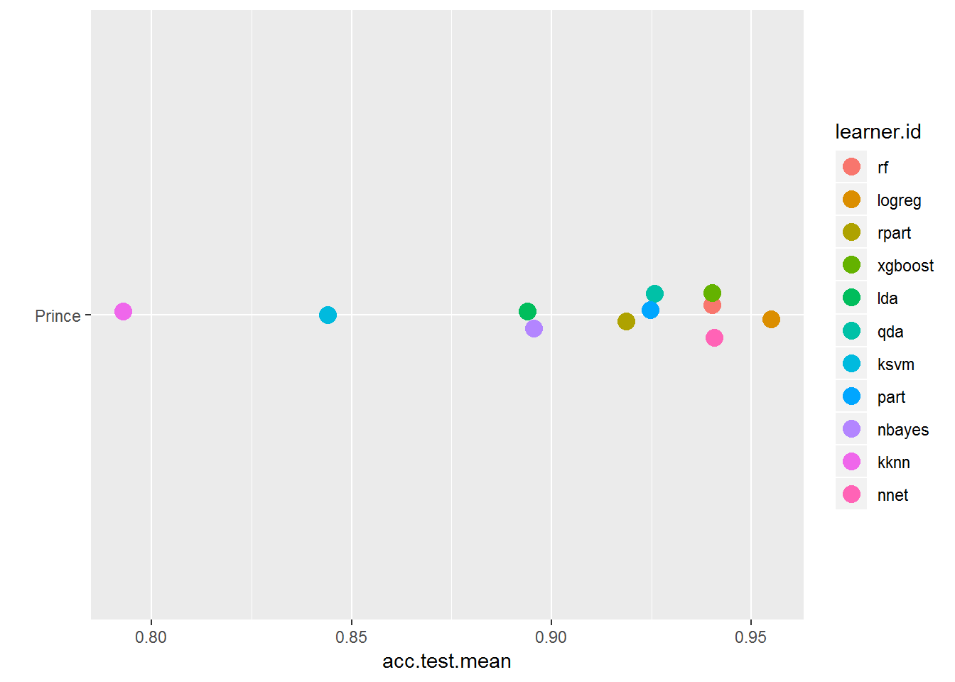
plotBMRSummary(bmr_prince)

 plotBMRBoxplots(bmr_prince, measure = acc, style = "violin", pretty.names = FALSE) +
  aes(color = learner.id) +
  ylab("Accuracy") +
  theme(strip.text.x = element_text(size = 8))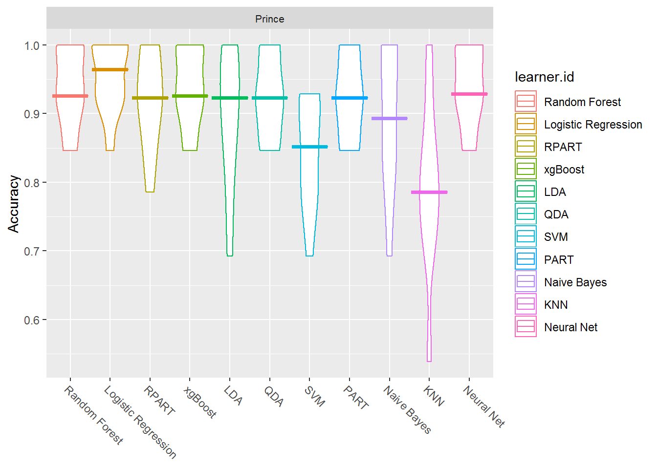

 #with knn so you can see the numbers
getBMRAggrPerformances(bmr_prince, as.df = TRUE) %>%
  select(ModelType = learner.id, Accuracy = acc.test.mean) %>%
  mutate(Accuracy = round(Accuracy, 4)) %>%
  arrange(desc(Accuracy)) %>%
  my_kable_styling("Validation Set Model Comparison")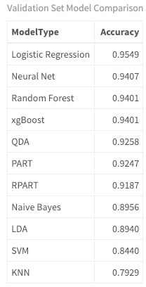

In predicting chart level, you are now working with a two class problem. There are only two options: charted or uncharted. When classifying genre, you had a multiclass problem where there were more than two possible classes. (Note this is different than a multi-label problem where an observation can have more than one class. That may be something to look into!). As a result of this being a binomial classification problem, I've added a couple of different algorithms: QDA and Logistic Regression. These two are more suited to two-class problems.

Logistic Regression is designed for binary results and models the probability that an observation (song) belongs to a particular category. It is based on a threshold that defaults to .5. For example, anything with greater than a .5 probability belongs to the target class, and anything below this threshold belongs to the other class. This threshold is adjustable. QDA is short for quadratic discriminant analysis and is more flexible for handling quadratic versus linear decision boundaries. Ok, it's not fair for me to throw out technical terms without more information, so please take the time to look at the data you have to work with, the algorithms that perform well, and investigate each one separately. I hope this analysis is enticing you to research the details!

The next step is to run your predictions and look at the classifications.

 predictions <- getBMRPredictions(bmr_prince)

calculateConfusionMatrix(predictions$Prince$`QDA`)$result %>%
  my_kable_styling("Logistic Regression Confusion Matrix: Rows are True, Columns are Predictions")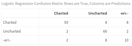

Misclassification

It is very easy to look at how the model classifies each individual song. With binary classification, there are quite a few measures to examine. For now, just look at the false positives - i.e., which songs were predicted to chart when in fact, they did not break into the Top 100.

 false_positives <- as.data.frame(predictions$Prince$`QDA`) %>%
  filter(truth == "Uncharted" & response == "Charted")

song_summary$id <- seq_len(nrow(song_summary))
song_summary %>%
  inner_join(false_positives) %>%
  inner_join(prince_charted_data) %>%
  select(song, response, truth, peak, album, year) %>%
  my_kable_styling("False Positive Prince Songs")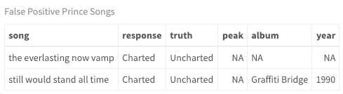

Where's the Test?

Even though you used cross-validation when training your model, you should always run that model against a separate dataset (like you did with genre above). I have left that as an exercise for you and hope that you will leave feedback on your results. For this to be a true test of the predictive power behind the lyric analysis, the most realistic results would come from a separate artist also in the pop-rock genre like Prince. Another factor is the time period. These songs charted in mostly the 70s, 80s, and 90s, so an artist of the same time period is critical. Or, choose your own artists for training and test data and see what you get!

Conclusion

In this tutorial, you have built a model to predict the genre of a song based entirely on lyrics. You used supervised machine learning classification algorithms and trained models on a set of five different artists and five different genres. By using the mlr framework, you created tasks, learners and resampling strategies to train and then tune a model(s). Then you ran your model against an unseen test dataset of different artists. You were able to identify which algorithms work better with the default settings, and eventually, predict the genre of new songs that your model has never seen.

With respect to lyric analysis, it should be clear that even though the music industry (and the Billboard Charts) have pre-defined genres for each artist, your analysis implies that according to lyrics, songs span genres and there is not usually a one-to-one relationship. (Being a songwriter myself, my genre tag-line is "funkified, acoustic, rockin' soul!"). You were also able to use the same techniques to model whether a song will hit the charts based entirely on lyrics with decent accuracy on training data. Your mission is now to apply that knowledge to your own datasets!

I've enjoyed working with you throughout this entire three-part (four tutorials) series of articles on lyric analysis. Hopefully, you have come to appreciate the complexity of working with this type of text and the subtleties involved with lyrics compared to other forms of text (i.e., non-fiction). I hope you have learned new skills and are inspired to use your own data to capture insights for new topics of interest to you. Machine learning is an exciting field, and as a new or experienced data scientist, creativity, inspiration, and persistence will set you apart from the norm. So remember to think outside of the quadrilateral parallelogram and enjoy your learning adventure!

"I put my foot on the starting line, and took off into a brand new day. I blew a kiss into the wind, closed my eyes and kicked the fear away. - Debbie Liske, New Day"

(By the way, I have written over 100 songs of my own and ran that last model on my music. It predicted 35 of my songs should have hit the charts! If only I had known about this technique sooner!! Maybe my next article should be on how to use lyric analysis to write a hit song based on current day artists...)

Appendix

Topics for Further Analysis

I briefly touched upon the topics below and encourage you to spend time gaining a deeper understanding of each one.

• Repeat building your models over several passes and partition your data separately each time.
• Understand the concepts behind each algorithm and why some work better with certain datasets.
• Review the different aspects of performance measurement and why some are more relevant than others depending on the use case.
• Learn how to tune the hyperparameters for the different types of models
• Dive into resampling (cross-validation and bootstrapping) and understand its purpose.
• Consider other packages than simply mlr for more rounded knowledge
• Check out miscellaneous research papers and what is happening in the field of lyric analysis.

Please ask any questions in the comment section!

Here are the links to the datasets:

• five_sources_data_balanced.csv
• five_sources_data_test.csv
• explicit_words.csv
• prince_data_balanced.csv