PySpark Tutorial: Getting Started with PySpark

What is PySpark?

PySpark is an interface for Apache Spark in Python. With PySpark, you can write Python and SQL-like commands to manipulate and analyze data in a distributed processing environment. Using PySpark, data scientists manipulate data, build machine learning pipelines, and tune models.

Most data scientists and analysts are familiar with Python and use it to implement machine learning workflows. PySpark allows them to work with a familiar language on large-scale distributed datasets. Apache Spark can also be used with other data science programming languages like R. If this is something you are interested in learning, the Introduction to Spark with sparklyr in R course is a great place to start.

RDDs vs DataFrames in PySpark

PySpark gives you two ways to represent distributed data. Understanding which to use is one of the first questions a new PySpark user faces.

For the vast majority of work — including everything in this tutorial — DataFrames are the right choice. Spark's Catalyst query optimizer rewrites DataFrame operations into efficient execution plans automatically, giving you performance benefits you'd have to implement by hand with RDDs. Use RDDs only when you need direct control over partitioning or are working with data that doesn't fit a tabular schema.

Why Use PySpark?

PySpark is the go-to choice for processing big data because it combines Python's accessibility with Spark's distributed computing power. Here's how it compares to alternatives:

The reason companies choose to use a framework like PySpark is because of how quickly it can process big data. It is faster than libraries like Pandas and Dask, and can handle larger amounts of data than these frameworks. If you had over petabytes of data to process, for instance, Pandas and Dask would fail but PySpark would be able to handle it easily.

While it is also possible to write Python code on top of adistributed system like Hadoop, many organizations choose to use Spark insteadand use the PySpark API since it is faster and can handle real-time data. With PySpark, you can write code to collect data from a source that is continuously updated, while data can only be processed in batch mode with Hadoop. 

Apache Flink is a distributed processing system that has a Python API called PyFlink, and is actually faster than Spark in terms of performance. However, Apache Spark has been around for a longer period of time and has better community support, which means that it is more reliable. 

PySpark also provides fault tolerance: if a node fails mid-job, Spark reconstructs lost data using RDD lineage information.The framework also has in-memory computation and is stored in random access memory (RAM). It can run on a machine that does not have a hard-drive or SSD installed.

How to Install PySpark

Here's how to install PySpark locally or in a cloud environment. 

Prerequisites

Before beginning the installation, ensure you have the following prerequisites installed:

• Java 11 or later (Java 17 recommended)
• Python 3.7 or later
• Jupyter Notebook 

Note: If you're using cloud-based platforms like DataLab or Databricks, you can skip the local installation as PySpark comes pre-installed.

Installing PySpark

Open a Python file in your Jupyter Notebook and run the following lines of code in the first cell:

!pip install pyspark

Alternatively, you can follow along with this end-to-end PySpark installation guide to get the software installed on your device.

End-to-end Machine Learning PySpark Tutorial

Now that you have PySpark up and running, we will show you how to execute an end-to-end customer segmentation project using the library. 

Customer segmentation is a marketing technique companies use to identify and group users who display similar characteristics. For instance, if you visit Starbucks only during the summer to purchase cold beverages, you can be segmented as a “seasonal shopper” and enticed with special promotions curated for the summer season.

Data scientists usually build unsupervised machine learning algorithms, such as K-Means clustering or hierarchical clustering, to perform customer segmentation. These models are great at identifying similar patterns between user groups that often go unnoticed by the human eye.

In this tutorial, we will use K-Means clustering to perform customer segmentation on the e-commerce dataset.

By the end of this tutorial, you will be familiar with the following concepts:

• Reading CSV files with PySpark

• Exploratory Data Analysis with PySpark

• Grouping and sorting data

• Performing arithmetic operations

• Aggregating datasets

• Data Pre-Processing with PySpark

• Working with datetime values

• Type conversion

• Joining two data frames

• The rank() function

• PySpark Machine Learning

• Creating a feature vector

• Standardizing data

• Building a K-Means clustering model

• Interpreting the model

Step 1: Creating a SparkSession

A SparkSession is an entry point into all functionality in Spark, and is required if you want to build a dataframe in PySpark. Run the following lines of code to initialize a SparkSession: 

from pyspark.sql import SparkSession  # add this import


spark = (
    SparkSession.builder
    .appName("DataCamp PySpark Tutorial")
    .config("spark.memory.offHeap.enabled", "true")
    .config("spark.memory.offHeap.size", "10g")
    .getOrCreate()
)

Using the code above, we built a Spark session and set a name for the application. Then, the data was cached in off-heap memory to avoid storing it directly on disk, and the amount of memory was manually specified.

Step 2: Creating the DataFrame

We can now read the dataset. You can download the sample e-commerce dataset from our PySpark Read CSV tutorial or use your own CSV file:

df = spark.read.csv("datacamp_ecommerce.csv", header=True, escape='"', inferSchema=True)

Note that we defined an escape character to avoid commas in the .csv file when parsing.

Let’s take a look at the head of the DataFrame using the show() function:

df.show(5,0)

The DataFrame consists of 8 variables:

1. InvoiceNo: The unique identifier of each customer invoice.

2. StockCode: The unique identifier of each item in stock.

3. Description: The item purchased by the customer.

4. Quantity: The number of each item purchased by a customer in a single invoice.

5. InvoiceDate: The purchase date.

6. UnitPrice: Price of one unit of each item.

7. CustomerID: Unique identifier assigned to each user.

8. Country: The country from which the purchase was made.

Step 3: Exploratory data analysis

Now that we have seen the variables present in this dataset, let’s perform some exploratory data analysis to further understand these data points:

1. Let’s start by counting the number of rows in the DataFrame:

df.count()  # Answer: 2,500

1. How many unique customers are present in the DataFrame?

df.select('CustomerID').distinct().count() # Answer: 95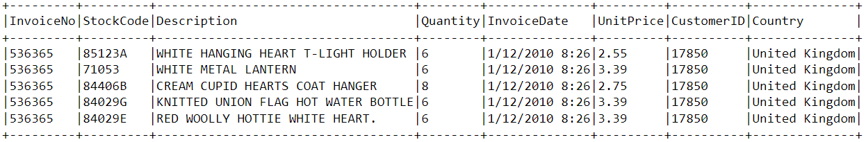

1. What country do most purchases come from?

To find the country from which most purchases are made, we need to use the groupBy() clause in PySpark:

from pyspark.sql.functions import *
from pyspark.sql.types import *

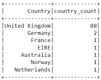
df.groupBy('Country').agg(countDistinct('CustomerID').alias('country_count')).show()

The following table will be rendered after running the code above:

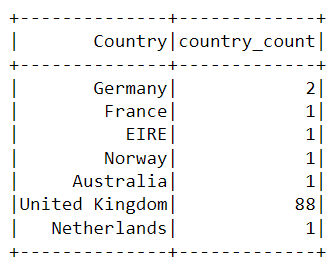
Almost all the purchases on the platform were made from the United Kingdom, and only a handful were made from countries like Germany, Australia, and France. 

Notice that the data in the table above isn’t presented in the order of purchases. To sort this table, we can include the orderBy() clause:

df.groupBy('Country').agg(countDistinct('CustomerID').alias('country_count')).orderBy(desc('country_count')).show()

The output displayed is now sorted in descending order:

1. When was the most recent purchase made by a customer on the e-commerce platform?

To find when the latest purchase was made on the platform, we need to convert the InvoiceDate column into a timestamp format and use the max() function in PySpark:

df = df.withColumn(
    "date",
    coalesce(
        to_timestamp(col("InvoiceDate"), "yy/MM/dd HH:mm"),
        to_timestamp(col("InvoiceDate"), "yyyy-MM-dd HH:mm:ss"),
        to_timestamp(col("InvoiceDate"))  # best-effort fallback
    )
)
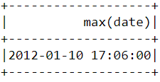
df.select(max("date")).show()

You should see the following table appear after running the code above:

1. When was the earliest purchase made by a customer on the e-commerce platform?

Similar to what we did above, the min() function can be used to find the earliest purchase date and time:

df.select(min("date")).show()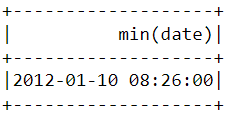

Notice that the most recent and earliest purchases were made on the same day, just a few hours apart. This means that the dataset we downloaded contains information of only purchases made on a single day.

Step 4: Data pre-processing

Now that we have analyzed the dataset and have a better understanding of each data point, we need to prepare the data to feed into the machine learning algorithm.

Let’s take a look at the head of the data frame once again to understand how the pre-processing will be done:

df.show(5,0)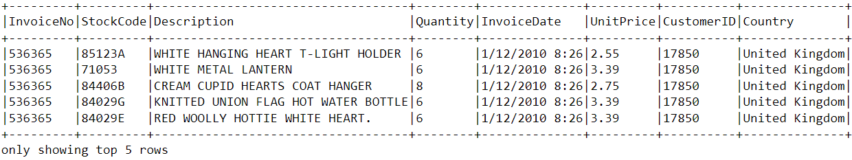

From the dataset above, we need to create multiple customer segments based on each user’s purchase behavior. 

The variables in this dataset are in a format that cannot be easily ingested into the customer segmentation model. These features individually do not tell us much about customer purchase behavior.

Due to this, we will use the existing variables to derive three new informative features - recency, frequency, and monetary value (RFM).

RFM is commonly used in marketing to evaluate a client’s value based on their:

1. Recency: How recently has each customer made a purchase?
2. Frequency: How often have they bought something?
3. Monetary Value: How much money do they spend on average when making purchases?

We will now preprocess the data frame to create the above variables.

Recency

First, let’s calculate the value of recency - the latest date and time a purchase was made on the platform. This can be achieved in two steps:

i) Assign a recency score to each customer

We will subtract every date in the data frame from the earliest date. This will tell us how recently a customer was seen in the data frame. A value of 0 indicates the lowest recency, as it will be assigned to the person who was seen making a purchase on the earliest date.

df = df.withColumn("from_date", to_timestamp(lit("12/1/10 08:26"), "yy/MM/dd HH:mm"))
df2 = df.withColumn("recency", col("date").cast("long") - col("from_date").cast("long"))


w = Window.partitionBy("CustomerID").orderBy(desc("recency"))
df2 = df2.withColumn("rn", row_number().over(w)).filter(col("rn") == 1).drop("rn")

ii) Select the most recent purchase

One customer can make multiple purchases at different times. We need to select only the last time they were seen buying a product, as this is indicative of when the most recent purchase was made: 

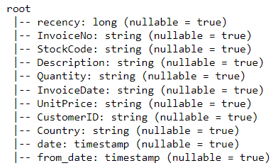
df2 = df2.join(df2.groupBy('CustomerID').agg(max('recency').alias('recency')),on='recency',how='leftsemi')

Let’s look at the head of the new data frame. It now has a variable called “recency” appended to it:

df2.show(5,0)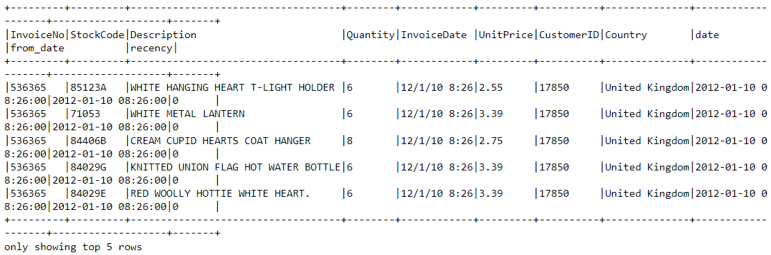

An easier way to view all the variables present in a PySpark DataFrame is to use its printSchema() function. This is the equivalent of the info() function in Pandas:

df2.printSchema()

The output rendered should look like this:

Frequency

Let’s now calculate the value of frequency - how often a customer buys something on the platform. To do this, we just need to group by each CustomerID and count the number of items they purchased. For more advanced grouping techniques, see our PySpark groupBy tutorial:

df_freq = df2.groupBy('CustomerID').agg(count('InvoiceDate').alias('frequency'))

Look at the head of this new DataFrame we just created:

df_freq.show(5,0)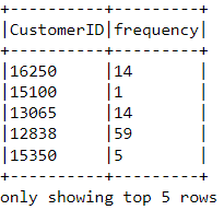

There is a frequency value appended to each customer in the DataFrame. This new DataFrame only has two columns, and we need to join it with the previous one. Learn more about different join types in our PySpark Joins tutorial:

df3 = df2.join(df_freq,on='CustomerID',how='inner')

Let’s print the schema of this DataFrame:

df3.printSchema()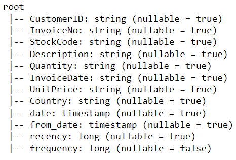

Monetary Value

Finally, let’s calculate monetary value - the total amount spent by each customer in the DataFrame. There are two steps to achieving this:

i) Find the total amount spent in each purchase:

Each CustomerID comes with variables called Quantity and UnitPrice for a single purchase:

To get the total amount spent by each customer in one purchase, we need to multiply Quantity with UnitPrice:

m_val = df3.withColumn(
    "TotalAmount",
    col("Quantity").cast("double") * col("UnitPrice").cast("double")
)

ii) Find the total amount spent by each customer:

To find the total amount spent by each customer overall, we just need to group by the CustomerID column and sum the total amount spent:

m_val = m_val.groupBy('CustomerID').agg(sum('TotalAmount').alias('monetary_value'))

Merge this DataFrame with all the other variables:

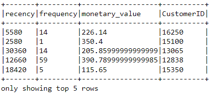
finaldf = m_val.join(df3,on='CustomerID',how='inner')

Now that we have created all the necessary variables to build the model, run the following lines of code to select only the required columns and drop duplicate rows from the DataFrame:

finaldf = finaldf.select(['recency','frequency','monetary_value','CustomerID']).distinct()

Look at the head of the final DataFrame to ensure that the pre-processing has been done accurately:

Standardization

Before building the customer segmentation model, let’s standardize the DataFrame to ensure that all the variables are around the same scale:

from pyspark.ml.feature import VectorAssembler, StandardScaler


assemble = VectorAssembler(
    inputCols=["recency", "frequency", "monetary_value"],
    outputCol="features"
)
assembled_data = assemble.transform(finaldf)


scale = StandardScaler(inputCol="features", outputCol="standardized")
data_scale = scale.fit(assembled_data)
data_scale_output = data_scale.transform(assembled_data)

Run the following lines of code to see what the standardized feature vector looks like:

data_scale_output.select('standardized').show(2,truncate=False)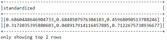

These are the scaled features that will be fed into the clustering algorithm.

If you’d like to learn more about data preparation with PySpark, take this feature engineering course on DataCamp.

Step 5: Building the machine learning model

Now that we have completed all the data analysis and preparation, let’s build the K-Means clustering model. 

The algorithm will be created using PySpark’s machine learning API.

i) Finding the number of clusters to use

When building a K-Means clustering model, we first need to determine the number of clusters or groups we want the algorithm to return. If we decide on three clusters, for instance, then we will have three customer segments.

The most popular technique used to decide on how many clusters to use in K-Means is called the “elbow method.”

This is done by running the K-Means algorithm for a range of cluster counts and visualizing the model results for each cluster. The plot will have an inflection point that looks like an elbow, and we just pick the number of clusters at this point.

Read this DataCamp K-Means clustering tutorial to learn more about how the algorithm works.

Let’s run the following lines of code to build a K-Means clustering algorithm from 2 to 10 clusters:

from pyspark.ml.clustering import KMeans
from pyspark.ml.evaluation import ClusteringEvaluator
import numpy as np

cost = np.zeros(10)

evaluator = ClusteringEvaluator(
    predictionCol="prediction",
    featuresCol="standardized",
    metricName="silhouette",
    distanceMeasure="squaredEuclidean"
)


ks = range(2, 10)
cost = np.zeros(len(ks))


for idx, k in enumerate(ks):
    km = KMeans(featuresCol="standardized", k=k)
    model = km.fit(data_scale_output)
    output = model.transform(data_scale_output)
    cost[idx] = model.summary.trainingCost   # WSSSE

With the code above, we have successfully built and evaluated a K-Means clustering model with 2 to 10 clusters. The results have been placed in an array, and can now be visualized in a line chart:

import pandas as pd
import pylab as pl
df_cost = pd.DataFrame(cost)  # cost has 8 values, one per k in range(2, 10)
df_cost.columns = ["cost"]
new_col = range(2, 10)
df_cost.insert(0, 'cluster', new_col)
pl.plot(df_cost.cluster, df_cost.cost)
pl.xlabel('Number of Clusters')
pl.ylabel('Score')
pl.title('Elbow Curve')
pl.show()

The code above will render the following chart:

ii) Building the K-Means Clustering Model

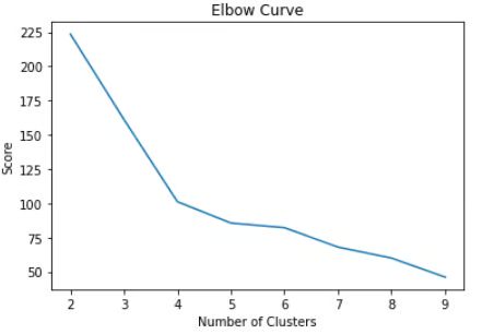
From the plot above, we can see that there is an inflection point that looks like an elbow at four. Due to this, we will proceed to build the K-Means algorithm with four clusters:

KMeans_algo=KMeans(featuresCol='standardized', k=4)
KMeans_fit=KMeans_algo.fit(data_scale_output)

iii) Making predictions

Let’s use the model we created to assign clusters to each customer in the dataset:

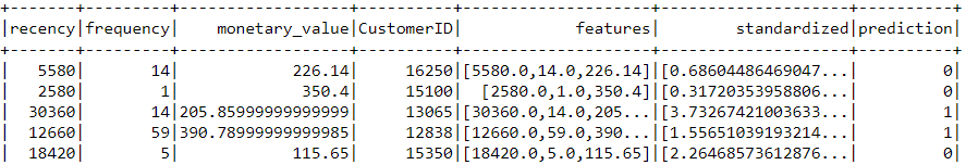
preds=KMeans_fit.transform(data_scale_output)

preds.show(5,0)

Notice that there is a “prediction” column in this DataFrame that tells us which cluster each CustomerID belongs to:

Step 6: Cluster Analysis

The final step in this entire tutorial is to analyze the customer segments we just built.

Run the following lines of code to visualize the recency, frequency, and monetary value of each CustomerIDin the DataFrame:

import matplotlib.pyplot as plt
import seaborn as sns

df_viz = preds.select('recency','frequency','monetary_value','prediction')
df_viz = df_viz.toPandas()
avg_df = df_viz.groupby(['prediction'], as_index=False).mean()

rfm_columns = ['recency', 'frequency', 'monetary_value']

for metric in rfm_columns:
    sns.barplot(x='prediction', y=metric, data=avg_df)
    plt.show()

The code above will render the following plots:

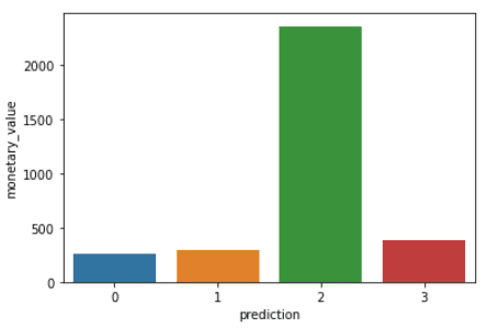
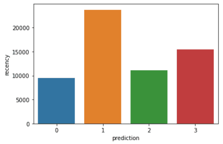
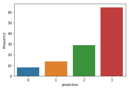
Here is an overview of characteristics displayed by customers in each cluster:

• Cluster 0: Customers in this segment display low recency, frequency, and monetary value. They rarely shop on the platform and are low-potential customers who are likely to stop doing business with the e-commerce company.
• Cluster 1: Users in this cluster display high recency but haven’t been seen spending much on the platform. They also don’t visit the site often. This indicates that they might be newer customers who have just started doing business with the company.
• Cluster 2: Customers in this segment display medium recency and frequency and spend a lot of money on the platform. This indicates that they tend to buy high-value items or make bulk purchases.
• Cluster 3: The final segment comprises users who display high recency and make frequent purchases on the platform. However, they don’t spend much on the platform, which might mean that they tend to select cheaper items in each purchase.

To go beyond the predictive modeling concepts covered in this course, you can take the Machine Learning with PySpark course on DataCamp.

Learning PySpark From Scratch: Next Steps

Now that you've completed this tutorial, here are the recommended next steps based on your goals:

If you managed to follow along with this entire PySpark tutorial, congratulations! You have now successfully installed PySpark onto your local device, analyzed an e-commerce dataset, and built a machine learning algorithm using the framework.

One caveat of the analysis above is that it was conducted with 2,500 rows of ecommerce data collected on a single day. The outcome of this analysis can be solidified if we had a larger amount of data to work with, as techniques like RFM modeling are usually applied onto months of historical data.

However, you can take the principles learned  in this article and apply them to a wide variety of larger datasets in the unsupervised machine learning space.

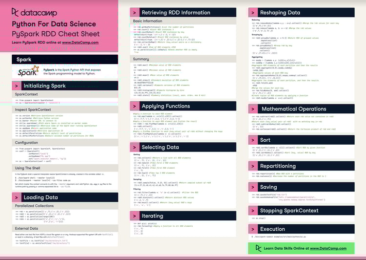
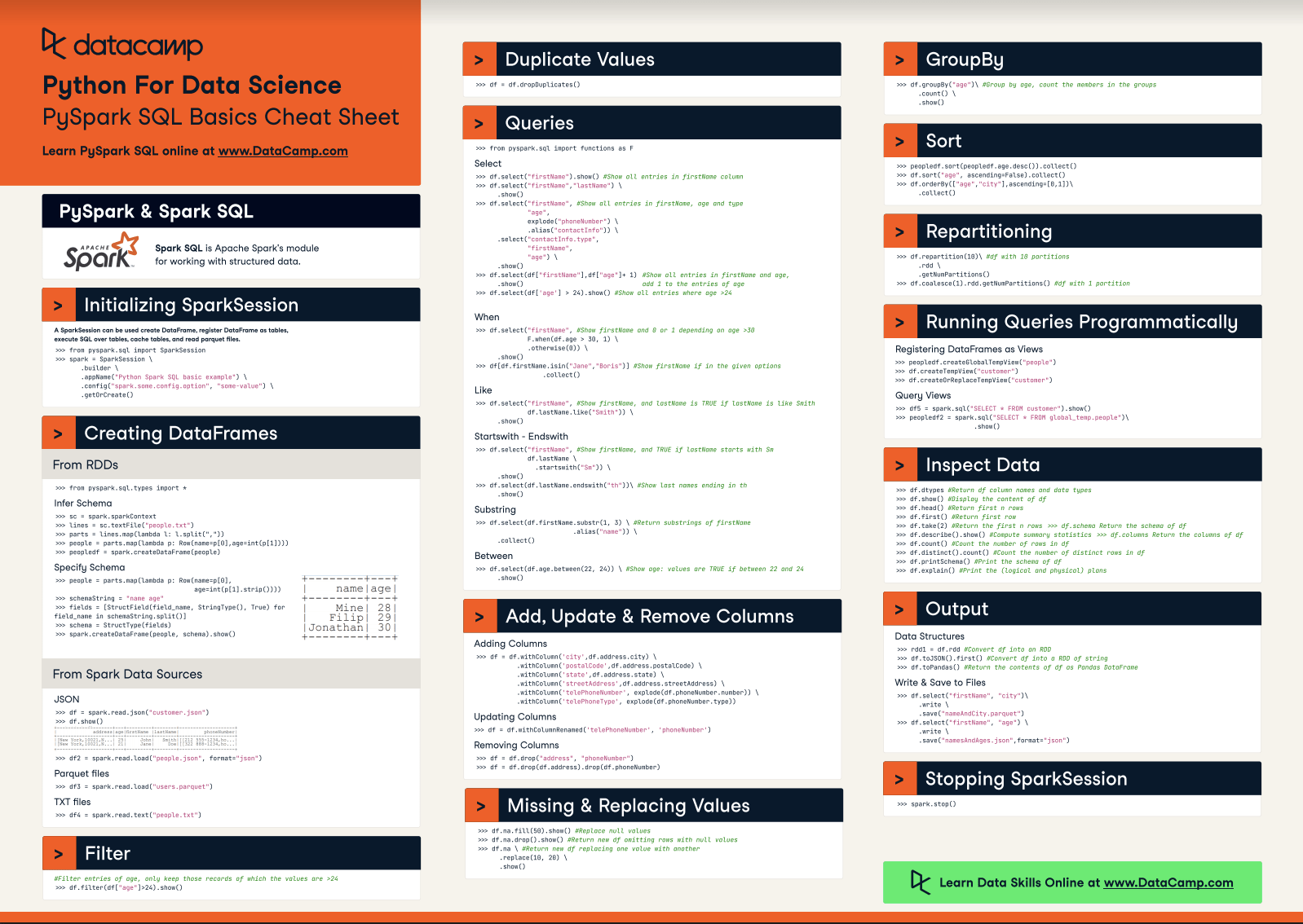
Check out this cheat sheet by DataCamp tolearn more about PySpark’s syntax and its modules.

Finally, if you’d like to go beyond the concepts covered in this tutorial and learn the fundamentals of programming with PySpark, you can take the Big Data with PySpark learning track on DataCamp. This track contains a series of courses that will teach you to do the following with PySpark:

• Data Management, Analysis, and Pre-processing
• Building and Tuning Machine Learning Pipelines
• Big Data Analysis 
• Feature Engineering 
• Building Recommendation Engines

Final thoughts

PySpark is the right tool when your data outgrows what a single machine can handle. The RFM customer segmentation project in this tutorial walks through the full workflow: loading data, exploratory analysis, feature engineering, and ML. These are patterns you'll reuse on much larger datasets in production.

One honest caveat: this example uses 2,500 rows from a single day of transactions. PySpark handles that comfortably. The real payoff from a distributed setup comes when you're working with months of transaction history across millions of events — that's when the in-memory execution and fault tolerance actually matter.

To keep building, our Big Data with PySpark track covers data engineering pipelines, recommendation engines, and production ML in a structured sequence. For teams, DataCamp for Business offers learning paths tailored to data engineering roles. Request a demo to learn more.