Course
Introduction to R
4 hr
3M
While the field of machine learning advances swiftly with the development of increasingly more sophisticated techniques, little attention has been given to high-dimensional multi-task problems that require the simultaneous prediction of multiple responses. This tutorial will show you the power of the Graph-Guided Fused LASSO (GFLASSO) in predicting multiple responses under a single regularized linear regression framework.
In supervised learning, one usually aims at predicting a dependent or response variable from a set of explanatory variables or predictors over a set of samples or observations. Regularization methods introduce penalties that prevent overfitting of high-dimensional data, particularly when the number of predictors exceeds the number of observations. These penalties are added to the objective function so that the coefficient estimates of uninformative predictors (that contribute little to the minimization of the error) are minimized themselves. The least absolute shrinkage and selection operator (LASSO) [1] is one such method.
Compared to a ordinary least squares (OLS), the LASSO is capable of shrinking coefficient estimates (β) to exactly zero, thereby ruling out uninformative predictors and performing feature selection, via
$$argmin_\beta \sum_n(y_n-\hat{y_n})^2+\lambda\sum_{j}|\beta_{j}|$$
where n and j denote any given observation and predictor, respectively. The residual sum of squares (RSS), the sole term used in OLS, can equivalently be written in the algebraic form $RSS = \sum_n(y_n-\hat{y_n})^2 = (y-X\beta)^T.(y-X\beta)$. The LASSO penalty is λ∑j|βj|, the L1 norm of the coefficient estimates weighted by λ.
What if you set to predict multiple related responses at once, from a common set of predictors? While effectively you could fare well with multiple independent LASSO models, one per response, you would be better off by coordinating those predictions with the strength of association among responses. This is because such coordination cancels out the response-specific variation that includes noise - the key strength of the GFLASSO.
A good example is provided in the original article, in which the authors resolve the associations between 34 genetic markers and 53 asthma traits in 543 patients [2].
Let X be a matrix of size n × p , with n observations and p predictors and Y a matrix of size n × k, with the same n observations and k responses, say, 1390 distinct electronics purchase records in 73 countries, to predict the ratings of 50 Netflix productions over all 73 countries.
Models well poised for modeling pairs of high-dimensional datasets include orthogonal two-way Partial Least Squares (O2PLS), Canonical Correlation Analysis (CCA) and Co-Inertia Analysis (CIA), all of which involving matrix decomposition [3]. Additionally, since these models are based on latent variables (that is, projections based on the original predictors), the computational efficiency comes at a cost of interpretability.
However, this trade-off does not always pay off, and can be reverted with the direct prediction of k individual responses from selected features in X, in a unified regression framework that takes into account the relationships among the responses.
Mathematically, the GFLASSO borrows the regularization of the LASSO [1] discussed above and builds the model on the graph dependency structure underlying Y, as quantified by the k × k correlation matrix (that is the 'strength of association' that you read about earlier). As a result, similar (or dissimilar) responses will be explained by a similar (or dissimilar) subset of selected predictors.
More formally, and following the notation used in the original manuscript [2], the objective function of the GFLASSO is

where, over all k responses, ∑k(yk − X**βk)T.(yk − X**βk) provides the RSS and λ∑k∑j|βj**k| the regularization penalty borrowed from the LASSO, weighted by the parameter λ and acting on the coefficients β of every individual predictor j. The novelty of the GFLASSO lies in
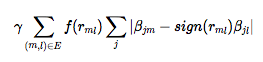
the fusion penalty weighted by γ that ensures the absolute difference between the coefficients βj**m and βj**l, from any predictor j and pair of responses m and l, will be the smaller (resp. larger) the more positive (resp. more negative) their pairwise correlation, transformed or not, f(rm**l). This fusion penalty favours globally meaningful variation in the responses over noise from each of them. When the pairwise correlation is close to zero, it does nothing, in which case you are left with a pure LASSO. This underlying correlation structure of all k responses, which can be represented as a weighted network structure, defaults to the absolute correlation, f(rm**l)=|rm**l| but can be transformed to create GFLASSO variants with any user-specified function, such as
with plenty more room for innovation. Although 2. is much less computationally intensive compared to 1. and the default absolute correlation [2], it does require a predefined cutoff, for example, τ = 0.8.
To sum up, to fit a GFLASSO model you will need a predictor matrix X, a response matrix Y and a correlation matrix portraying the strength of association between all pairs of responses in Y. Note that the GFLASSO yields a p × k matrix of β, unlike the LASSO (p × 1), and this coefficient matrix carries the associations between any given response k and predictor j.
Kris Sankaran and I have been working on an experimental R package that implements the GFLASSO alongside cross-validation and plotting methods. We have recently implemented multi-threading using the doParallel package, rendering much faster cross-validation (CV) routines.
To run GFLASSO in R you will need to install devtools, load it and install the gflasso package from my GitHub repository. The demonstration will be conducted on a dataset contained in the package bgsmtr. I also recommend installing corrplot and pheatmap to visualize the results.
# Install the packages if necessary
#install.packages("devtools")
#install.packages("bgsmtr")
#install.packages("corrplot")
#install.packages("pheatmap")
library(devtools)
library(bgsmtr)
library(corrplot)
library(pheatmap)
#install_github("monogenea/gflasso")
library(gflasso)You can easily run the simulation outlined in the help page for the CV function cv_gflasso(). By default, the CV computes the root mean squared error (RMSE) across a single repetition of a 5-fold CV, over all possible pairs between λ ∈ {0, 0.1, 0.2, ..., 0.9, 1} and γ ∈ {0, 0.1, 0.2, ..., 0.9, 1}, the tuning grid.
Note that user-provided error functions will also work!
Besides the inherent statistical assumptions and speed performance, the choice of tuning grid ranges depends largely on mean-centering and unit-variance scaling all columns in X and Y, so please make sure you do so beforehand.
In the following example you will not need it, since you will draw random samples from a standard normal distribution. You can try deriving the fusion penalty from an unweighted correlation network, with a cutoff of r > 0.8:
?cv_gflasso
set.seed(100)
X <- matrix(rnorm(100 * 10), 100, 10)
u <- matrix(rnorm(10), 10, 1)
B <- u %*% t(u) + matrix(rnorm(10 * 10, 0, 0.1), 10, 10)
Y <- X %*% B + matrix(rnorm(100 * 10), 100, 10)
R <- ifelse(cor(Y) > .8, 1, 0)
system.time(testCV <- cv_gflasso(X, Y, R, nCores = 1))

## [1] 1.826146 1.819430 1.384595 1.420058 1.408619

##    user  system elapsed
##  45.808   3.070  55.271

system.time(testCV <- cv_gflasso(X, Y, R, nCores = 2))

## [1] 1.595413 1.492953 1.469917 1.366832 1.441642

##    user  system elapsed
##  22.231   1.698  26.441

cv_plot_gflasso(testCV)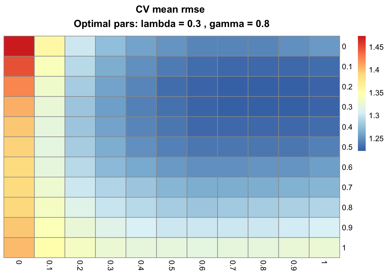
The optimal values of λ (rows) and γ (columns) that minimize the RMSE in this simulation, 0.3 and 0.8 respectively, do capture the imposed relationships.
Tip: Try re-running this example with a different metric, the coefficient of determination (R2). One key advantage of using R2 is that it ranges from 0 to 1.
Keep in mind that when you provide a custom goodness-of-fit function err_fun(), you have to define whether to maximize or minimize the resulting metric using the argument err_opt.
The following example aims at maximizing R2, using a weighted association network with squared correlation coefficients (i.e. f(rm**l)=rm**l2). If you have more than 2 cores, you might as well change the nCores argument and give it a boost!
# Write R2 function
R2 <- function(pred, y){
      cor(as.vector(pred), as.vector(y))**2
}

# X, u, B and Y are still in memory
R <- cor(Y)**2

# Change nCores, if you have more than 2, re-run CV
testCV <- cv_gflasso(X, Y, R, nCores = 2, err_fun = R2, err_opt = "max")

## [1] 0.6209191 0.7207394 0.7262781 0.7193907 0.6303187

cv_plot_gflasso(testCV)
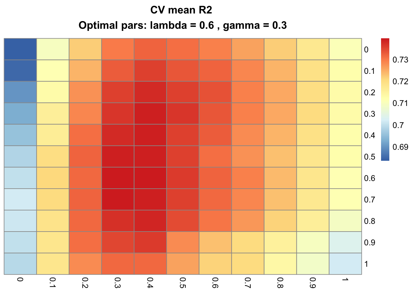
The optimal parameters λ and γ are now 0.6 and 0.3, respectively.
Also, note that cv_gflasso objects comprise single lists with four elements: the mean ($mean) and standard error ($SE) of the metric over all cells of the grid, the optimal λ and γ parameters ($optimal) and the name of the goodness-of-fit function ($err_fun). The cross-validated model from the present example clearly favors both sparsity (λ) and fusion (γ).
Finally, bear in mind you can fine-tune additional parameters, such as the Nesterov's gradient convergence threshold δ and the maximum number of iterations by passing delta_conv and iter_max to additionalOpts, respectively. These will be used in the following example.
To demonstrate the simplicity and robustness of the GFLASSO in a relatively high-dimensional problem, you will next model the bgsmtr_example_data datasets obtained from the Alzheimer’s Disease Neuroimaging Initiative (ADNI-1) database.
This is a 3-element list object, part of the bgsmtr package that consists of 15 structural neuromaging measures and 486 single nucleotide polymorphisms (SNPs, genetic markers) determined from a sample of 632 subjects. Importantly, the 486 SNPs cover 33 genes deemed associated with Alzheimer's disease.
Your task is to predict the morphological, neuroimaging measures from the SNP data, leveraging the correlation structure of the former.
Let's start by organizing the data and exploring the inter-dependencies among all neuroimaging features:
data(bgsmtr_example_data)
str(bgsmtr_example_data)

## List of 3
##  $ SNP_data     : int [1:486, 1:632] 2 0 2 0 0 0 0 1 0 1 ...
##   ..- attr(*, "dimnames")=List of 2
##   .. ..$ : chr [1:486] "rs4305" "rs4309" "rs4311" "rs4329" ...
##   .. ..$ : chr [1:632] "V1" "V2" "V3" "V4" ...
##  $ SNP_groups   : chr [1:486] "ACE" "ACE" "ACE" "ACE" ...
##  $ BrainMeasures: num [1:15, 1:632] 116.5 4477.9 28631.9 34.1 -473.4 ...
##   ..- attr(*, "dimnames")=List of 2
##   .. ..$ : chr [1:15] "Left_AmygVol.adj" "Left_CerebCtx.adj" "Left_CerebWM.adj" "Left_HippVol.adj" ...
##   .. ..$ : chr [1:632] "V1" "V2" "V3" "V4" ...

# Transpose, so that samples are distributed as rows, predictors / responses as columns
SNP <- t(bgsmtr_example_data$SNP_data)
BM <- t(bgsmtr_example_data$BrainMeasures)

# Define dependency structure
DS <- cor(BM)

# Plot correlation matrix of the 15 neuroimaging measures
corrplot(DS)
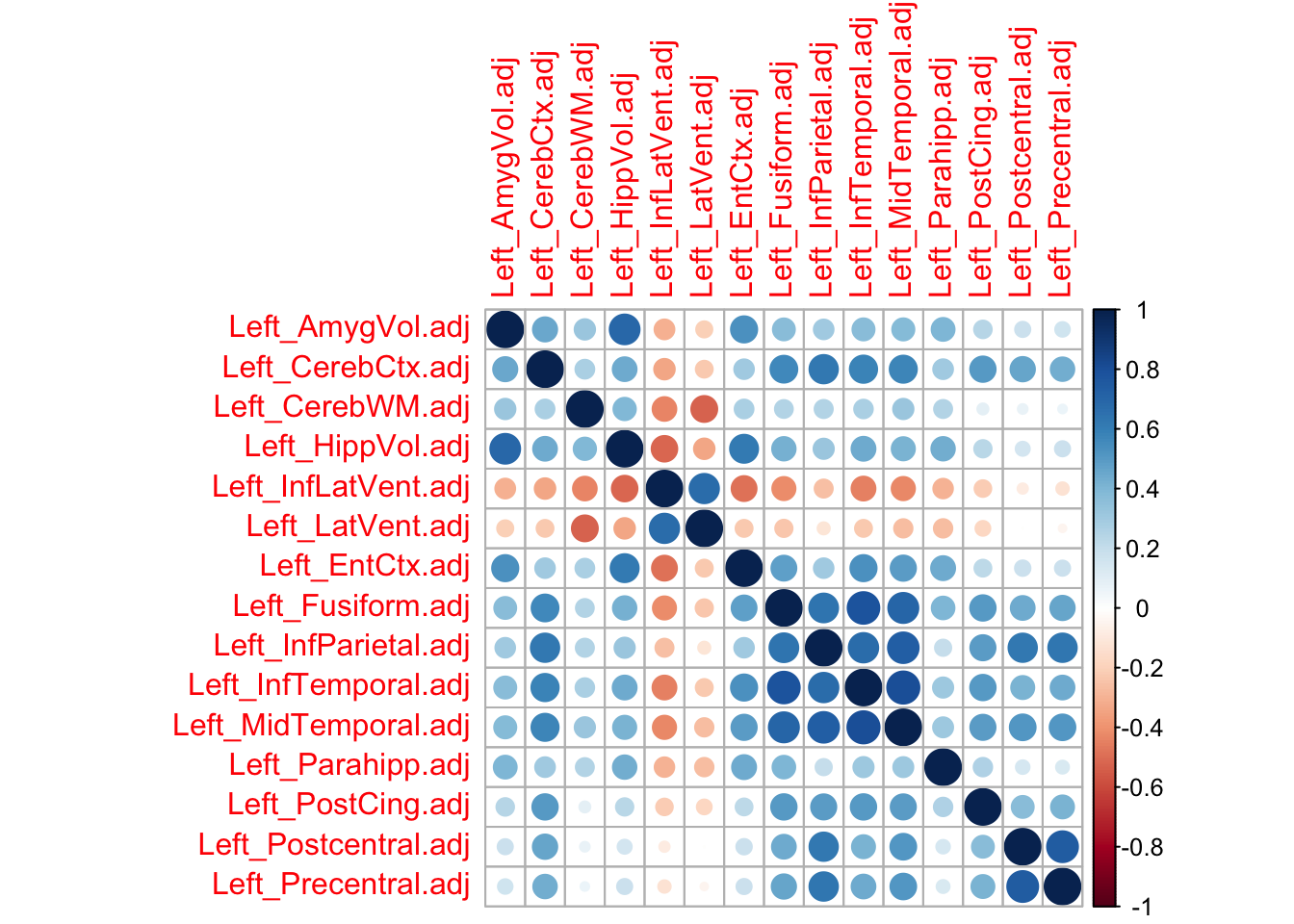
The figure above points to the interdependencies among the neuroimaging features. Try now cross-validating the GFLASSO (can take up to a couple of hours in a laptop!) and determine SNP-neuroimaging associations.
Note that in the example below, the convergence tolerance and the maximum number of iterations are specified. Feel free to try different values on your own!
system.time(CV <- cv_gflasso(X = scale(SNP), Y = scale(BM), R = DS, nCores = 2,
                 additionalOpts = list(delta_conv = 1e-5, iter_max = 1e5)))

## [1] 1.550294 1.471637 1.470133 1.514425 1.504215

##      user    system   elapsed
##  2611.492   323.441 51129.936

cv_plot_gflasso(CV)
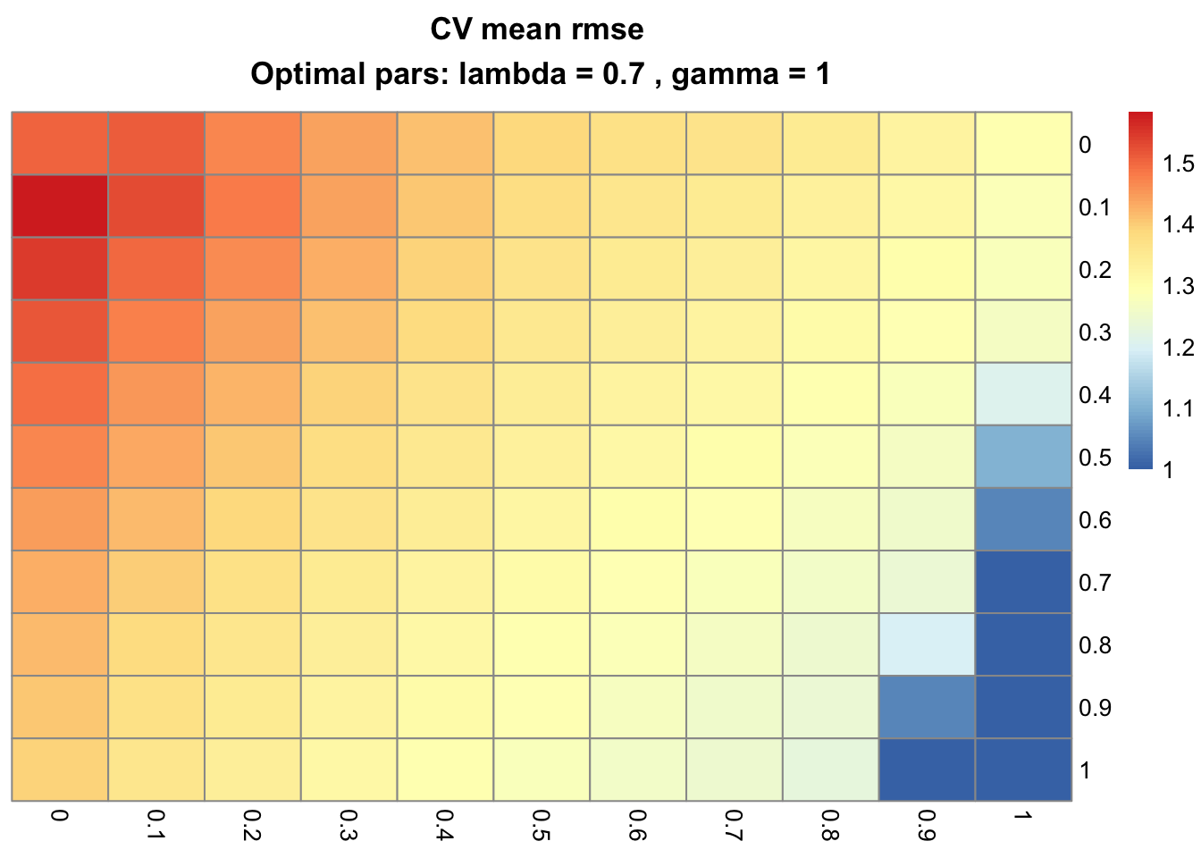
By challenging the GFLASSO with pure LASSO models (γ = 0, first column), a pure fusion least squares (λ = 0, first row) and OLS (γ = 0 and λ = 0, top-left cell), we can conclude the present example is best modeled with non-zero penalty weights and consequently, with the full GFLASSO. Take the optimal CV parameters (λ = 0.7 and γ = 1) to build a GFLASSO model and interpret the resulting coefficient matrix:
gfMod <- gflasso(X = scale(SNP), Y = scale(BM), R = DS, opts = list(lambda = CV$optimal$lambda,
                                                                    gamma = CV$optimal$gamma,
                                                                    delta_conv = 1e-5,
                                                                    iter_max = 1e5))
colnames(gfMod$B) <- colnames(BM)
pheatmap(gfMod$B, annotation_row = data.frame("Gene" = bgsmtr_example_data$SNP_groups,
                                              row.names = rownames(gfMod$B)),
         show_rownames = F)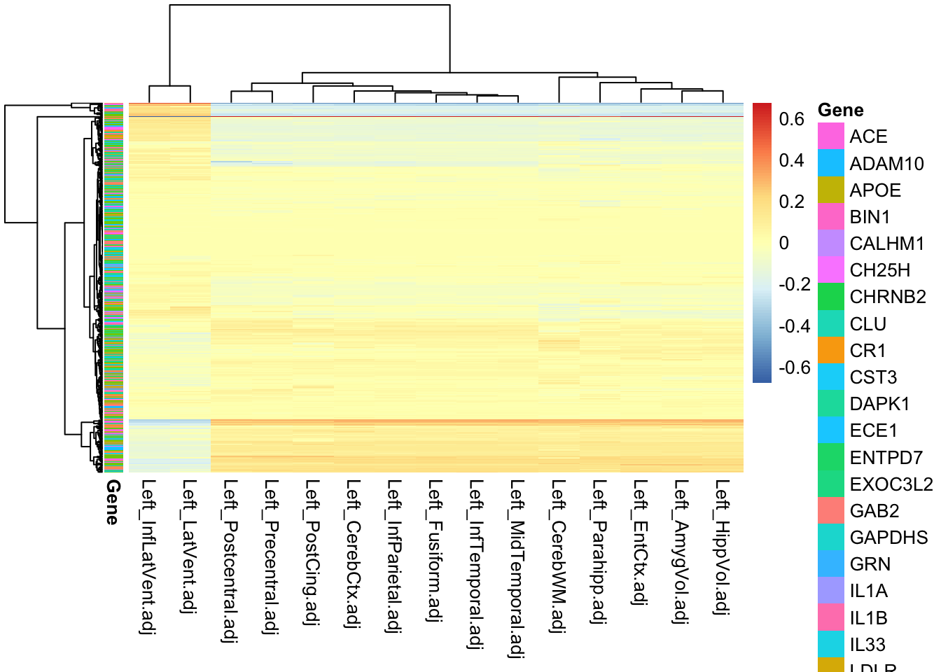
The figure above depicts a very large proportion of coefficients with zero or near-zero values. Although there is no obvious clustering of SNPs with respect to the genes (see row-wise annotation, note the legend is incomplete), there are clear associations between certains SNPs and traits.
In order to ascertain the existence of a non-random predictive mechanism, you could next repeat the procedure after permutation of the values in either X or Y. Experimental work could help elucidate causality and mechanisms from selected SNPs. For example, SNPs that affect protein sequence and structure, disrupting the clearance of the β-Amyloid plaques that underlie Alzheimer's disease.
The GFLASSO employs both regularization and fusion when modeling multiple responses, thereby facilitating the identification of associations between predictors (X) and responses (Y). It is best used when handling high-dimensional data from very few observations, since it is much slower than contending methods. Sparse conditional Gaussian graphical models [4] and Bayesian group-sparse multi-task regression model [5], for example, might be favoured chiefly for performance gains. Nevertheless, the GFLASSO is highly interpretable. I recently used the GFLASSO in a omics-integrative approach to uncover new lipid genes in maize [6].
Check out DataCamp's Regularization Tutorial: Ridge, Lasso and Elastic Net.
Kris and I will be very happy to hear from you. This project is currently maintained by Kris under the repo krisrs1128/gflasso and through mine, although under frequent changes, at monogenea/gflasso. Write me anytime (francisco.lima278@gmail.com), all feedback is welcome.
Happy coding!
R Courses
Course
Course
Course
Tutorial
Zoumana Keita
Tutorial
Karlijn Willems
Tutorial
Michał Oleszak
Tutorial
Vidhi Chugh
Tutorial
DataCamp Team
Tutorial
Salin Kc