Logistic Regression in R Tutorial

Logistic regression is a simple but powerful model to predict binary outcomes. That is, whether something will happen or not. It's a type of classification model for supervised machine learning.

Logistic regression is used in in almost every industry—marketing, healthcare, social sciences, and others—and is an essential part of any data scientist’s toolkit.

To make the most from this tutorial you need a basic working knowledge of R. It also helps to know about a related model type, linear regression. Read the Linear Regression in R Tutorial to find out about that.

An Overview of Logistic Regression

Suppose you want to predict whether today is going to be a sunny day or not. There are two possible outcomes: "sunny" or "not sunny". The outcome variable is also known as a "target variable" or a "dependent variable".

There are many variables that could influence the outcome such as ‘temperature the day before’, ‘air pressure’ etc. the influencing variables are known as features, independent variables, or predictors—all these terms mean the same thing. 

Other examples include whether a customer will buy your product or not, whether an email is spam or not, whether a transaction is fraudulent or not, and whether a drug will cure a patient or not.  

How does logistic regression work?

Logistic regression finds the best possible fit between the predictor and target variables to predict the probability of the target variable belonging to a labeled class/category. 

Linear regression tries to find the best straight line that predicts the outcome from the features. It forms an equation like

y_predictions = intercept + slope * features

and uses optimization to try and find the best possible values of intercept and slope.

Logistic regression works similarly, except it performs regression on the probabilities of the outcome being a category. It uses a sigmoid function (the cumulative distribution function of the logistic distribution) to transform the right-hand side of that equation.

y_predictions = logistic_cdf(intercept + slope * features)

Again, the model uses optimization to try and find the best possible values of intercept and slope.

Since the algorithm for logistic regression is very similar to the equation for linear regression, it forms part of a family of models called "generalized linear models". This is why logistic regression has "regression" in its name, even though it is a classification model.

The sigmoid function resembles an S-shaped curve in the image below. It takes the real numbered input values and converts them between 0 to 1 (by shrinking from both sides, i.e., the negative values to 0 and very high positive ones to 1). Furthermore, the cut-off threshold is the overlaying deciding factor that bins the output into categories or classes when applied on top of these probabilities.

The complex concepts are best understood when explained with examples, so let us pick up an analogy to register the working of the LR algorithm. Let’s assume that the LR model is tasked to identify a fraudulent transaction by looking at multiple fraud indicators, such as the user’s location, purchase amount, IP address, etc. The objective is to determine the likelihood of whether a given transaction is legitimate or fraudulent – which constitutes the target variable.

The model assigns weights to the predictors based on how they impact the target variable and combines them to calculate the normalized score or probability of fraud. 

The Dataset

We would use a direct marketing campaign dataset by a Portuguese banking institution using phone calls. The campaign aims to sell subscriptions of a bank term deposit represented by the variable y (subscription or no subscription). The objective of the logistic regression model is to predict whether a customer would buy a subscription or not based on the predictor variables, aka attributes of the customer, such as demographic information.

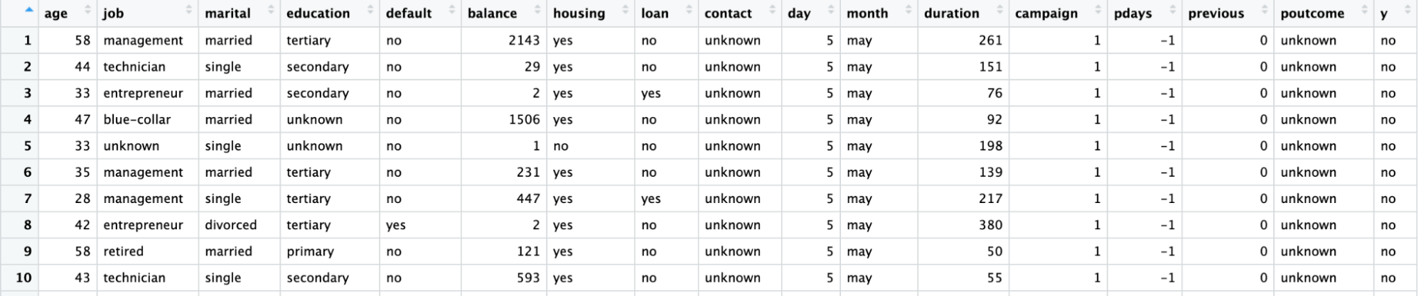
The data dictionary for this dataset and many other useful datasets can be found on the Datacamp’s website.

Logistic Regression Workflow

The full machine learning workflow is covered in the A Beginner's Guide to The Machine Learning Workflow infographic. Here we'll focus on data preparation and modeling steps. In particular, we'll cover:

• Splitting the data into training and testing sets
• Fitting (training) the model
• Making predictions
• Evaluating the model performance
• Hyperparameter tuning

Logistic Regression Packages

In R, there are two popular workflows for modeling logistic regression: base-R and tidymodels.

The base-R workflow models is simpler and includes functions like glm() and summary() to fit the model and generate a model summary.

The tidymodels workflow allows easier management of multiple models and a consistent interface for working with different model types.

This tutorial will use the tidymodels workflow.

Visualize the Data

Import the tidymodels package by calling the library() function. 

The dataset is in a CSV file with European-style formatting (commas for decimal places and semi-colons for separators). We'll read it with read_csv2() from the readr package. 

Convert the target variable, y, to a factor variable for modeling. 

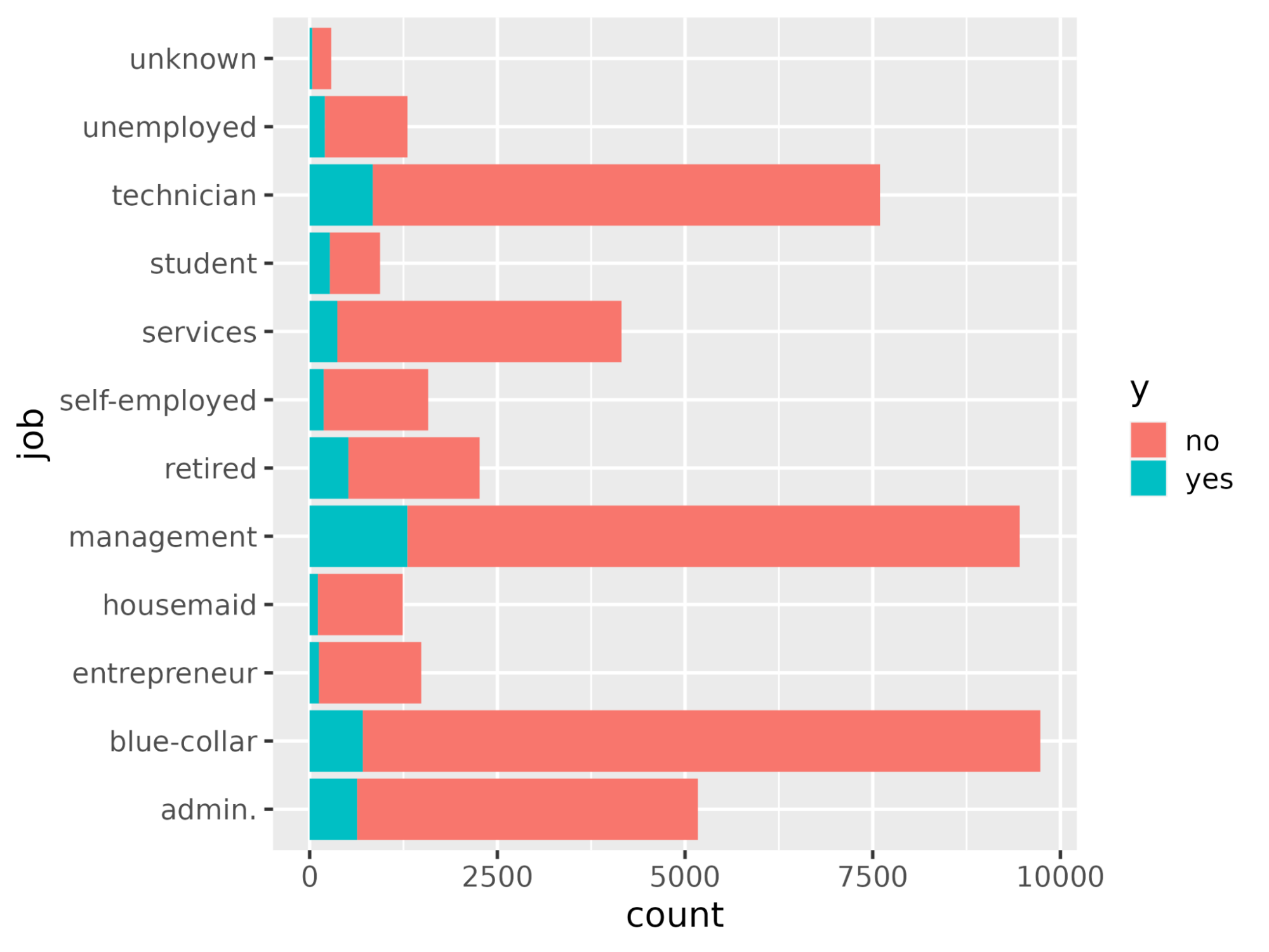
Using the ggplot() function plot the count of each job occupation with respect to y.

library(readr)
library(tidymodels)

# Read the dataset and convert the target variable to a factor
bank_df <- read_csv2("bank-full.csv")
bank_df$y = as.factor(bank_df$y)

# Plot job occupation against the target variable
ggplot(bank_df, aes(job, fill = y)) +
    geom_bar() +
    coord_flip()

Splitting the Data

Let’s split the dataset into a training set for fitting the model and a test set for model evaluation to make sure the model thus trained works on an unseen dataset.

Splitting data into training and test set can be performed using the initial_split() function and the prop attribute defining the train data proportion.

# Split data into train and test
set.seed(421)
split <- initial_split(bank_df, prop = 0.8, strata = y)
train <- split %>% 
         training()
test <- split %>% 
        testing()

Fitting and Evaluating the Model

To create the model, declare a logistic_reg() model. This needs mixture and penalty arguments which control the amount of regularization. A mixture value of 1 denotes a lasso model and 0 denotes ridge regression. Values in between are also allowed. The penalty argument denotes the strength of the regularization.

Note that you need to pass "double" floating point numbers to the mixture and penalty

Set the "engine" (the backend software used to run the calculations) with set_engine(). There are several choices: The default engine is "glm", which performs a classical logistic regression. This is often favored by statisticians because you get p-values for each coefficient, making it easier to understand the importance of each coefficient.

Here's we'll use the "glmnet" engine. This is favored by machine learning scientists because it allows regularization, which can improve predictions, particularly if you have a lot of features. (In Python, the scikit-learn package defaults to including some regularization in logistic regression.)

Call the fit() method to train the model on the training data created in the previous step. This takes a formula for its first argument. On the left-hand side of the formula, you use the target variable (in this case y). On the right-hand side, you can include any features you like. A period means "use all the variables that weren't written on the left-hand side of the formula. For more information on writing formulae, read the R Formula Tutorial.

# Train a logistic regression model
model <- logistic_reg(mixture = double(1), penalty = double(1)) %>%
  set_engine("glmnet") %>%
  set_mode("classification") %>%
  fit(y ~ ., data = train)

# Model summary
tidy(model)

The output is shown below with the estimate column representing coefficients of the predictor.

# A tibble: 43 × 3
   term              estimate penalty
   <chr>                <dbl>   <dbl>
 1 (Intercept)      -2.59           0
 2 age              -0.000477       0
 3 jobblue-collar   -0.183          0
 4 jobentrepreneur  -0.206          0
 5 jobhousemaid     -0.270          0
 6 jobmanagement    -0.0190         0
 7 jobretired        0.360          0
 8 jobself-employed -0.101          0
 9 jobservices      -0.105          0
10 jobstudent        0.415          0
# ... with 33 more rows
# ℹ Use `print(n = ...)` to see more rows

Making predictions

Make predictions on the testing data using the predict() function. You have choice of the type of predictions.

• type = "class" returns the most likely target value for each observation. Here, it will return a "yes" or a "no" depending on whether the model thinks the client is likely to subscribe to a term deposit or not.
• type = "prob" returns the probability of each target value for each observation. Here, it will return a the probability of a "yes" and the probability of a "no" (which add up to one for each observation).

# Class Predictions
pred_class <- predict(model,
                      new_data = test,
                      type = "class")

# Class Probabilities
pred_proba <- predict(model,
                      new_data = test,
                      type = "prob")

Evaluate the model using the accuracy() function with truth argument as y and estimate the argument value to be the predictions from the previous step.

results <- test %>%
           select(y) %>%
           bind_cols(pred_class, pred_proba)

accuracy(results, truth = y, estimate = .pred_class)

Hyperparameter Tuning

Rather than passing specific values to the mixture and penalty arguments (the "hyperparameters"), you can optimize the predictive power of the model by tuning it. 

The idea is that you run the model lots of times with different values of the hyperparameters, and see which one gives the best predictions.

• In the logistic_reg() function, set the mixture and penalty arguments to a call to tune().
• Use the grid_regular() function to define a grid of possible values for mixture and penalty.
• The workflow() function creates an object to store the model details, which is needed when you run it many times. 
• Choose the best model using the select_best() function. You can pick from a choice of metrics that defines the "best" one. Here, we'll use the "receiver operating characteristic area under the curve" (ROC AUC) metric.

# Define the logistic regression model with penalty and mixture hyperparameters
log_reg <- logistic_reg(mixture = tune(), penalty = tune(), engine = "glmnet")

# Define the grid search for the hyperparameters
grid <- grid_regular(mixture(), penalty(), levels = c(mixture = 4, penalty = 3))

# Define the workflow for the model
log_reg_wf <- workflow() %>%
  add_model(log_reg) %>%
  add_formula(y ~ .)

# Define the resampling method for the grid search
folds <- vfold_cv(train, v = 5)

# Tune the hyperparameters using the grid search
log_reg_tuned <- tune_grid(
  log_reg_wf,
  resamples = folds,
  grid = grid,
  control = control_grid(save_pred = TRUE)
)

select_best(log_reg_tuned, metric = "roc_auc")

# A tibble: 1 × 3
       penalty mixture .config              
         <dbl>   <dbl> <chr>                
1 0.0000000001       0 Preprocessor1_Model01

More Evaluation Metrics

Using the best hyperparameters:

1. Let’s train a logistic regression model
2. Use it to generate predictions on test set
3. Create a confusion matrix using the true values, and the estimates

# Fit the model using the optimal hyperparameters
log_reg_final <- logistic_reg(penalty = 0.0000000001, mixture = 0) %>%
                 set_engine("glmnet") %>%
                 set_mode("classification") %>%
                 fit(y~., data = train)

# Evaluate the model performance on the testing set
pred_class <- predict(log_reg_final,
                      new_data = test,
                      type = "class")
results <- test %>%
  select(y) %>%
  bind_cols(pred_class, pred_proba)

# Create confusion matrix
conf_mat(results, truth = y,
         estimate = .pred_class)

Truth
Prediction   no  yes
       no  7838  738
       yes  147  320

You can calculate the precision (positive predictive value, the number of true positives divided by the number of predicted positives) with the precision() function.

precision(results, truth = y,
          estimate = .pred_class)

# A tibble: 1 × 3
  .metric   .estimator .estimate
  <chr>     <chr>          <dbl>
1 precision binary         0.914

Similarly, you can calculate the recall (sensitivity, the number of true positives divided by the number of actual positives) with the recall() function.

recall(results, truth = y,
          estimate = .pred_class)

# A tibble: 1 × 3
  .metric .estimator .estimate
  <chr>   <chr>          <dbl>
1 recall  binary         0.982

Let’s understand the variables impacting the subscription buying decision. In a logistic regression scenario, the coefficients decide how sensitive the target variable is to the individual predictors. The higher the value of coefficients the higher their importance is. Sort the variables in descending order of the absolute value of their coefficient values and display only the coefficients with an absolute value greater than 0.5.

coeff <- tidy(log_reg_final) %>% 
  arrange(desc(abs(estimate))) %>% 
  filter(abs(estimate) > 0.5)

# A tibble: 10 × 3
   term            estimate      penalty
   <chr>              <dbl>        <dbl>
 1 (Intercept)       -2.59  0.0000000001
 2 poutcomesuccess    2.08  0.0000000001
 3 monthmar           1.62  0.0000000001
 4 monthoct           1.08  0.0000000001
 5 monthsep           1.03  0.0000000001
 6 contactunknown    -1.01  0.0000000001
 7 monthdec           0.861 0.0000000001
 8 monthjan          -0.820 0.0000000001
 9 housingyes        -0.550 0.0000000001
10 monthnov          -0.517 0.0000000001

Plot the feature importance using the ggplot() function.

ggplot(coeff, aes(x = term, y = estimate, fill = term)) + geom_col() + coord_flip()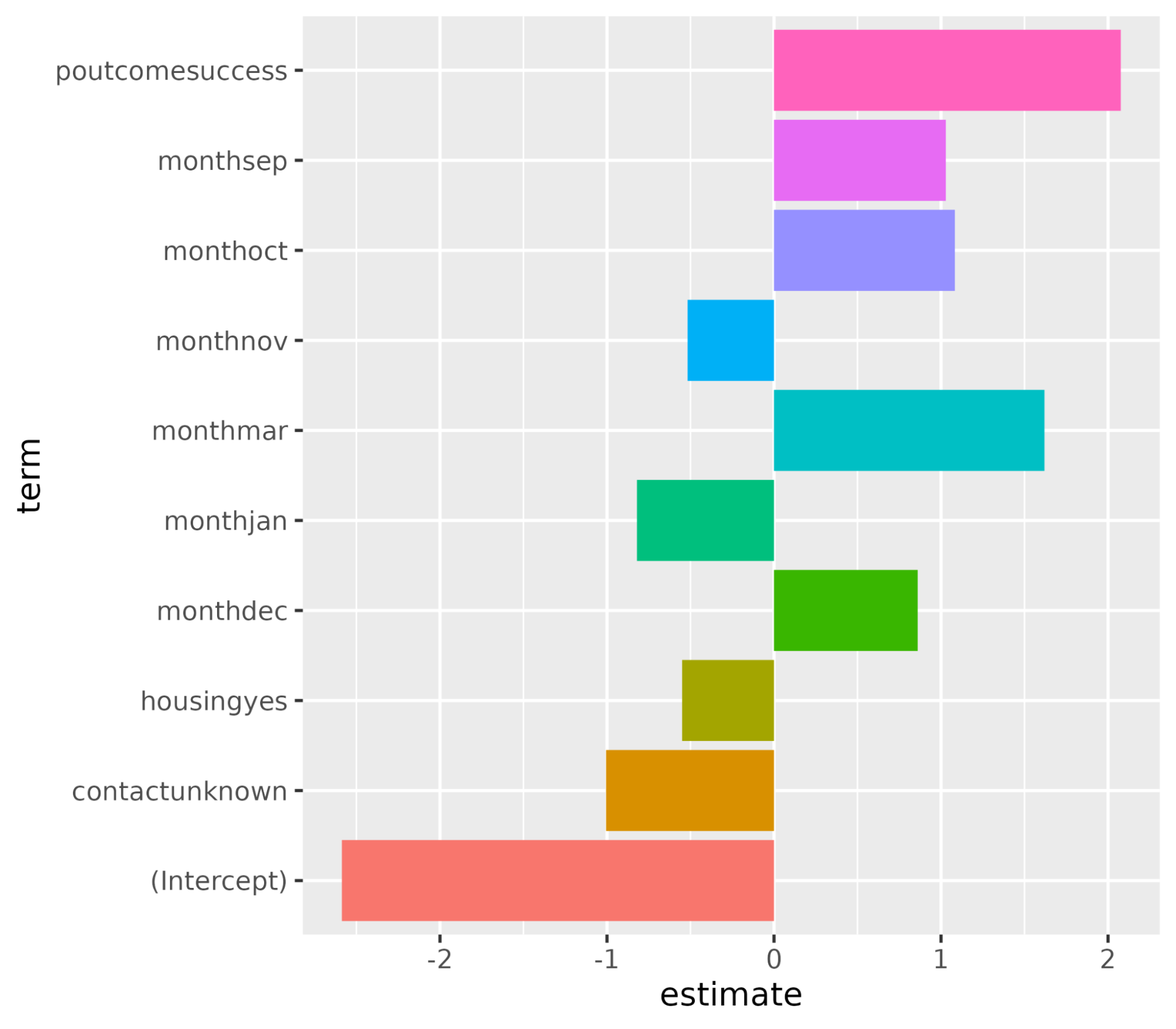

Take it to the Next Level

With this, we have reached toward the end of this tutorial that demonstrated how to train and evaluate a logistic regression model using the tidymodels package. It also covered how to interpret the model results and plot them like feature importance. 

If you are inquisitive about learning more about modeling AI models using tidymodels, do check out the course on Modeling with tidymodels in R. For modeling using the base-R approach, check out the Introduction to Regression in R, Intermediate Regression in R, and Generalized Linear Models in R courses.