Gurobi: Mathematical Optimization for Complex Problems

Basic solvers and trial-and-error methods struggle when variables scale up. Gurobi handles these complexities with speed and precision, solving problems in seconds that might otherwise take hours. That’s the difference between hoping for a feasible plan and mathematically proving you have the optimal one.

This tutorial guides you throughthe powerful commercial solver known as Gurobi. I will show you how to install the Python library, formulate your first model, and scale up to advanced problems like mixed-integer programming.

Understanding Mathematical Optimization and Gurobi's Role

Before writing code, it helps to understand what optimization really means. This context shows you when to use Gurobi instead of standard programming approaches.

What is mathematical optimization?

Mathematical optimization finds the best solution from all possible solutions. You define what "best" means (minimize cost, maximize profit, minimize time), what you control (decision variables), and what limits you face (constraints). The optimizer searches through feasible solutions to find the optimal one.

This differs from traditional programming, where you specify exact steps. With optimization, you describe the problem mathematically and let the solver figure out how to solve it. You're not writing "if this then that" logic, you're defining relationships and letting algorithms find the best values.

Gurobi's significance in optimization

Why Gurobi stands out

Gurobi consistently ranks as one of the fastest commercial optimizers available. Benchmarks show it solving large-scale problems 10-100 times faster than open-source alternatives. This speed matters when you're running optimization hourly or need results within strict time limits.

Industry adoption

Companies across logistics, finance, energy, and healthcare use Gurobi for production systems. FedEx optimizes delivery routes, while financial firms allocate billions in portfolios. Energy companies schedule power generation. These aren't academic exercises, they're systems handling real money and real constraints.

Solver capabilities

Gurobi handles linear programming (LP), mixed-integer programming (MIP), quadratic programming (QP), and more. It includes state-of-the-art algorithms like concurrent optimization, where multiple solution methods run in parallel and the fastest wins. You get reliability and speed without choosing algorithms manually.

Setting Up Gurobi

Installing Gurobi takes just a few steps. Once configured, it works seamlessly with Python.

Installation and setup

Download and install

Go to Gurobi's website and grab the installer for your OS. It includes the optimizer, the gurobipy interface, and documentation. Run the installer with default settings unless you need a custom path.

After installation, verify it worked:

import gurobipy as gp
print(f"Gurobi version: {gp.__version__}")

Here, we verify the installation by printing the version number. A successful print confirms your environment is ready.

Licensing options

Gurobi requires a license for anything beyond small test problems. Your options:

• Free trial license: 30-day evaluation. Request it from Gurobi's website with your work email.
• Academic license: Free for faculty and students. Verify your academic email for unlimited access, which is perfect for learning.
• Commercial license: Required for business. Pricing varies by scale. Named-user licenses suit individual data scientists, while floating licenses let teams share capacity.
• Cloud license: Pay-as-you-go. No upfront cost, just pay for what you use. Useful for occasional optimization tasks.

I use the academic license for learning and the commercial one for production. The trial gives you plenty of time to explore before committing.

Environment configuration

Python setup

Gurobi works with Python 3.7+. I recommend using a virtual environment to avoid conflicts:

python -m venv gurobi_env
gurobi_env\Scripts\activate
source gurobi_env/bin/activate
pip install gurobipy

These commands set up a clean workspace and pull in the library.

Jupyter Notebook integration

For interactive development, notebooks work great with Gurobi:

pip install jupyter
jupyter notebook
import gurobipy as gp
print("Gurobi ready!")

This snippet installs Jupyter, fires up the server, and runs a quick check to ensure Gurobi loads correctly within the notebook.

When NOT to use Gurobi

Gurobi is powerful, but not always the right choice.

• Simple problems: If you have 50 variables and basic linear constraints, free solvers like scipy.optimize.linprog or Excel Solver work fine.

• Cost: Commercial licenses are expensive. For non-critical internal tools, open-source options like CBC or GLPK (via PuLP) might suffice.

• Heuristics: If you need a "good enough" answer in milliseconds for a real-time game, heuristics (like genetic algorithms) often beat exact solvers.

Use Gurobi when problems are large (10k+ variables) or you need advanced features like quadratic constraints.

Platform compatibility

Gurobi runs on Windows, macOS, and Linux. Cloud environments like AWS, Azure, and Google Cloud support Gurobi through their marketplaces. I've deployed Gurobi models on all three major clouds without platform-specific issues.

Building Optimization Models

With Gurobi installed, let's build your first model. These core concepts apply to every problem you'll solve.

Key components of an optimization model

Every model has three essential parts:

Decision variables

These are the choices the optimizer makes. In production planning, this might be "units of Product A" and "units of Product B." You define the variables; Gurobi assigns the values.

Objective function

This is your goal, what you want to maximize or minimize. Maximize profit (3*product_a + 5*product_b) or minimize cost. You get one objective per model.

Constraints

These are your limits. You can't produce more than factory capacity or spend more than your budget. Constraints define which solutions are actually possible.

Formulation best practices

Use clear variable names. Instead of x[1], use produce_product_a. It saves you hours of debugging later, as I'll explain in the troubleshooting section.

Keep constraints simple. Breaking complex logic into smaller, simpler constraints makes your model easier to read and debug.

Modern Gurobi: The Matrix API

If you are coming from a data science background, loop-based modeling might feel slow. Gurobi 13.0+ offers a Matrix API that uses NumPy arrays, making model building 10-50x faster.

Here is how a bakery model looks using vectors:

import gurobipy as gp
import numpy as np

# Data
prices = np.array([2.0, 5.0])
resources = np.array([[0.5, 2.0], [1.0, 1.0]])
limits = np.array([100.0, 80.0])

model = gp.Model("bakery_matrix")
x = model.addMVar(shape=2, name="x")

model.setObjective(prices @ x, gp.GRB.MAXIMIZE)
model.addConstr(resources @ x <= limits, name="constraints")

model.optimize()

This A @ x <= b syntax is cleaner and standard for production systems.

Creating a simple linear programming model

Let's solve a practical problem: a bakery deciding how many loaves of bread and cakes to bake to maximize profit.

Problem setup:

- Bread profit: $2 | Flour: 0.5 kg

- Cake profit: $5 | Flour: 2 kg

- Flour available: 100 kg

- Oven capacity: 80 items

Here's the model:

import gurobipy as gp
from gurobipy import GRB

model = gp.Model("bakery_optimization")

bread = model.addVar(name="bread", vtype=GRB.CONTINUOUS, lb=0)
cake = model.addVar(name="cake", vtype=GRB.CONTINUOUS, lb=0)

model.setObjective(2 * bread + 5 * cake, GRB.MAXIMIZE)

model.addConstr(0.5 * bread + 2 * cake <= 100, name="flour_limit")
model.addConstr(bread + cake <= 80, name="oven_capacity")

model.optimize()

if model.status == GRB.OPTIMAL:
    print(f"Optimal profit: ${model.objVal:.2f}")
    print(f"Bake {bread.X:.2f} loaves of bread")
    print(f"Bake {cake.X:.2f} cakes")
else:
    print("No optimal solution found")

This code initializes the model, defines variables, and sets the profit objective. It applies the constraints we defined above and solves for the optimal plan.

Understanding solver logs

When you run model.optimize(), Gurobi prints a log. Here is how to read it:

Gurobi Optimizer version 13.0.0...
Presolve removed 0 rows and 0 columns
...
Explored 0 nodes (2 simplex iterations) in 0.01 seconds
Optimal objective  2.800000000e+02

• Presolve: Gurobi simplifies your problem before solving. "Removed rows" means it found redundant constraints.
• Simplex iterations: How many steps the algorithm took. High numbers on small problems might indicate formulation issues.
• Optimal objective: Your final result (e.g., $280 profit).
• Gap: For integer problems, this shows the difference between the best solution found so far and the theoretical best.

Watching the log helps you spot if a model is "stuck" or just working hard.

The concepts here scale directly. Whether you have 10 variables or 10,000, the pattern remains the same.

Advanced Problem Types Supported by Gurobi

Linear programming is just the start. Gurobi handles complex types that capture real-world nuances, including the new Non-Convex MINLP capabilities in version 13.0.

Mixed-integer linear programming

What makes it different

Mixed-integer programming (MIP) allows variables to be integers. You can't build 0.7 factories, so you need integer solutions.

Real-world applications

Facility location: Open a warehouse in City A? Yes (1) or No (0).

Production scheduling: Batch sizes often must be whole numbers.

Network design: Routing decisions are usually binary. Traffic flows through a link or it doesn't.

Example: facility location

import gurobipy as gp
from gurobipy import GRB

model = gp.Model("facility_location")

cities = ['CityA', 'CityB', 'CityC']
fixed_costs = {'CityA': 10000, 'CityB': 8000, 'CityC': 12000}

open_warehouse = model.addVars(cities, vtype=GRB.BINARY, name="open")

model.setObjective(
    gp.quicksum(fixed_costs[city] * open_warehouse[city] for city in cities),
    GRB.MINIMIZE
)

model.addConstr(gp.quicksum(open_warehouse[city] for city in cities) >= 2)

model.optimize()

print("Open warehouses in:")
for city in cities:
    if open_warehouse[city].X > 0.5:
        print(f"  {city}")

Here, we use binary variables to decide whether to open a warehouse. The model minimizes fixed costs while ensuring at least two facilities remain open.

Quadratic and nonlinear programming

Quadratic programming (QP)

When your objective includes squared terms or variable products, you have a QP. Portfolio optimization is a classic example because risk (variance) is quadratic.

Quadratically constrained programming (QCP)

Constraints can also be quadratic. Think of problems involving circles or curved boundaries.

Example: portfolio optimization

import gurobipy as gp
from gurobipy import GRB
import numpy as np

model = gp.Model("portfolio")

assets = ['StockA', 'StockB', 'StockC']
expected_returns = [0.12, 0.18, 0.10]

covariance = np.array([
    [0.04, 0.01, 0.02],
    [0.01, 0.09, 0.03],
    [0.02, 0.03, 0.05]
])

weights = model.addVars(len(assets), name="weight", lb=0, ub=1)

model.setObjective(
    gp.quicksum(expected_returns[i] * weights[i] for i in range(len(assets))),
    GRB.MAXIMIZE
)

model.addConstr(gp.quicksum(weights[i] for i in range(len(assets))) == 1)

risk_expr = gp.quicksum(
    covariance[i][j] * weights[i] * weights[j]
    for i in range(len(assets))
    for j in range(len(assets))
)
model.addConstr(risk_expr <= 0.05, name="risk_limit")

model.optimize()

print("Optimal portfolio allocation:")
for i, asset in enumerate(assets):
    print(f"{asset}: {weights[i].X * 100:.1f}%")

This setup tackles portfolio optimization. It maximizes returns while strictly capping the total risk (variance) using quadratic constraints.

Additional supported problem types

Second-order cone programming (SOCP)

Problems involving geometric constraints, such as defining a cone or a circular boundary, fall into this category. Common in robust optimization and engineering design.

Mixed-integer quadratic programming (MIQP)

Combines integer variables with quadratic objectives or constraints. Useful in discrete optimization with nonlinear relationships.

Gurobi supports all these types natively. You don't need to reformulate problems to fit a specific solver, Gurobi detects the problem type automatically and applies appropriate algorithms.

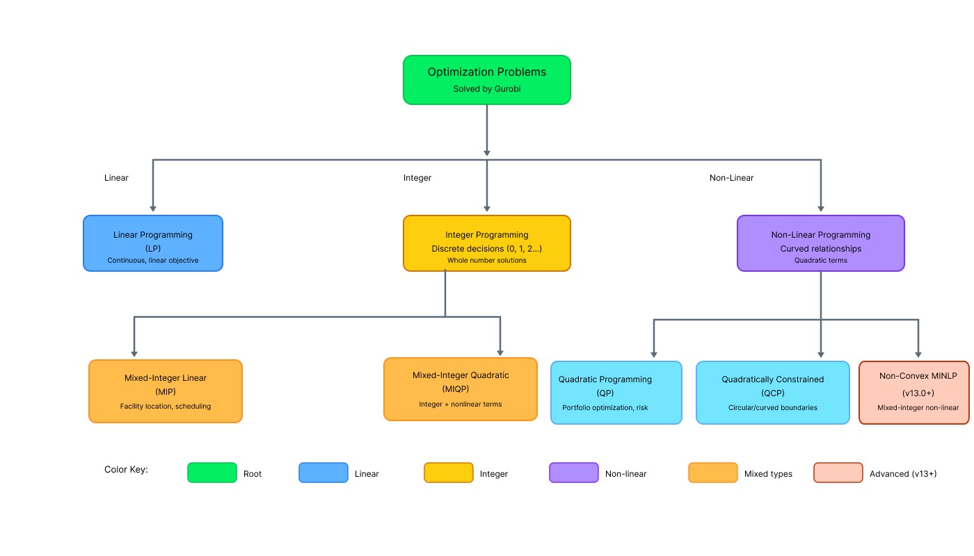
Optimization problem types supported by Gurobi. Image by Author.

Gurobi Algorithms and Their Applications

Algorithm selection

Gurobi picks algorithms automatically, but knowing the options helps when troubleshooting slow solves.

Method values:

• -1 (default): Let Gurobi decide

• 0: Primal simplex (good for most LPs)

• 1: Dual simplex (good when starting from infeasible)

• 2: Barrier (best for massive models or QP)

• 3: Concurrent (runs multiple methods, picks fastest)

• 4: Deterministic Concurrent

• 5: Deterministic Concurrent Simplex

• PDHG (First-Order Method: Gurobi 13.0 also includes PDHG, a gradient-based method ideal for massive LPs that fits on GPUs.

Check which ran by looking at the solver log (e.g., "Barrier solved model...").

When to override: If the default takes hours, try Barrier for huge models or Concurrent for unpredictable problems.

model.Params.Method = 2
model.Params.BarConvTol = 1e-8

This explicitly selects the Barrier method and tightens the tolerance, which helps when dealing with massive or sensitive datasets.

Utilizing Gurobi's Advanced Features

Once you master the basics, Gurobi offers powerful tools for enterprise-scale problems.

Distributed optimization

For massive models that take too long on a single machine, you can split the work. Gurobi's distributed optimization uses multiple computers to solve a single problem faster.

You designate one machine as the "manager" and others as "workers." The manager sends parts of the search tree to workers, who solve them in parallel. This is overkill for small models but essential for global supply chain or airline scheduling problems.

Multi-objective optimization

Real life rarely has just one goal. You might want to maximize profit and minimize environmental impact.

Gurobi handles this by letting you set priorities. You can tell it to "maximize profit first, then minimize waste without reducing profit by more than 10%." Alternatively, you can weight them: Objective = 0.7 * Profit - 0.3 * Waste.

# Multi-objective example
model.setObjectiveN(profit_expr, index=0, priority=2, name="Profit")
model.setObjectiveN(waste_expr, index=1, priority=1, name="Waste")

Real-time interaction and callbacks

Sometimes you want to intervene while Gurobi is solving. Callbacks let you run custom code at specific points, like every time a new solution is found.

I use callbacks to stop early if a solution is "good enough" or to inject custom heuristics that I know work for my specific data.

Cloud capabilities

Running optimization on your laptop is fine for development, but production often needs more power. Gurobi Cloud allows you to offload the heavy lifting to AWS, Azure, or Gurobi's own Instant Cloud. You pay only for the solve time, which is perfect for sporadic, heavy workloads.

Practical Modeling Best Practices

Writing efficient models requires strategy. Here are tips to keep your code clean and fast.

Model formulation strategies

Start simple, add complexity gradually

Don't build a 50-constraint model on day one. Start with the core logic, verify it, then refine. I've spent too much time debugging complex models only to find the error was in the basics.

Use meaningful variable and constraint names

x1 = model.addVar(name="x1")
model.addConstr(x1 + x2 <= 100, name="c1")

units_produced = model.addVar(name="units_produced")
model.addConstr(
    units_produced + units_stored <= warehouse_capacity,
    name="warehouse_capacity_limit"
)

Notice the difference: the second block clearly describes the business logic. As I mentioned earlier, this saves you debugging headaches.

Preprocess data

Validate your data before modeling. Check for missing values or impossible constraints. Finding data errors after a 3-hour solve is painful.

Scale your data appropriately

Gurobi handles numerical precision well, but extreme values cause trouble. If costs are in millions and quantities in thousandths, scale them to similar magnitudes:

# Instead of cost = 10000000 and quantity = 0.0001
# Scale to cost = 10 (in millions) and quantity = 100 (in 1/1000 units)

Numerical issues are rare in well-scaled models, common in poorly-scaled ones.

Numerical stability considerations

Gurobi uses floating-point arithmetic, which isn't infinite. If your constraint says x <= 1000000000 and your tolerance is 1e-6, you might get weird results.

Avoid "Big M" constraints like if y=0 then x <= 1,000,000,000. Instead, pick the smallest valid upper bound (e.g., total market size). Tighter bounds mean faster, more stable solves.

Warm starts and model modifications

You rarely solve a problem just once. Usually, new data arrives (e.g., updated demand).

Instead of rebuilding the model from scratch, use a warm start. You feed Gurobi the previous solution as a starting point. Since yesterday's optimal plan is likely close to today's, Gurobi can skip much of the search work.

# Warm start example
bread.Start = 40  # Start search assuming we bake 40 loaves

Programming Interfaces and Integration

Gurobi's Python API

We've used gurobipy because it's Pythonic. It supports operator overloading (x + y <= 5) and integrates directly with pandas and NumPy. It's the most popular way to use Gurobi for data science.

Integration with other languages

Production systems often run on C++, Java, or .NET for speed. Gurobi supports all of them. The concepts (Variables, Constraints, Objectives) are identical; only the syntax changes.

For cross-language workflows, I often prototype in Python (fast coding) and deploy in C++ (fast execution), using Gurobi's file formats (.mps or .lp) to move models between them.

Modeling language support

Gurobi also plugs into dedicated modeling languages like AMPL and GAMS, or even Excel.

- AMPL/GAMS: Great for purely mathematical researchers who don't want to write software code.

- Excel: Useful for quick prototypes or showing business stakeholders a model they can touch without installing Python.

Performance Optimization and Tuning

Tuning workflow

Don't tune randomly. Follow this process:

1. Measure baseline: Run with defaults, note solve time.

2. Set hard limits first: Production systems need TimeLimit.

3. Trade accuracy for speed: Only relax MIPGap if business tolerates it.

4. Test thread scaling: More threads ≠ faster (diminishing returns after 4-8).

# Example: Production deployment
model.Params.TimeLimit = 300  # Hard 5-min cutoff for API response
baseline_time = model.Runtime

if baseline_time > 240:  # If cutting it close
    model.Params.MIPGap = 0.02  # Accept 2% suboptimality
    # Business rationale: 2% cost increase < late delivery penalty

Performance benchmarks

Benchmarks show Gurobi consistently outperforms open-source solvers by orders of magnitude on hard MIP problems. While scipy handles small LPs fine, Gurobi shines when complexity scales. You can find comparative benchmarks on the Hans Mittelmann website, which tracks solver performance independently.

Debugging and troubleshooting

Model infeasibility

When Gurobi reports "Model is infeasible," your constraints conflict. No solution satisfies all of them simultaneously.

Find the conflicting constraints:

model.computeIIS()
model.write("infeasible.ilp")

print("Conflicting constraints:")
for c in model.getConstrs():
    if c.IISConstr:
        print(f"  {c.ConstrName}: {c.ConstrExpr}")

This calculates the Irreducible Inconsistent Subsystem (IIS) and prints exactly which constraints are fighting each other.

Unbounded models

An unbounded model means the objective can improve infinitely. Usually indicates missing constraints.

Check:

- Did you bound all variables? addVar(lb=0, ub=1000)

- Are constraints correctly formulated?

- Is the objective function correct?

Using solver logs

Enable detailed logging to see what Gurobi is doing:

model.Params.OutputFlag = 1
model.Params.LogToConsole = 1
model.Params.LogFile = "gurobi.log"

This enables verbose output and saves a copy to a local file, giving you a detailed history of the solve process.

Handling data

In real apps, data comes from files, not hardcoded lists.

import pandas as pd

# Load data
df = pd.read_csv("facility_costs.csv")
fixed_costs = dict(zip(df['city'], df['fixed_cost']))

# Validate BEFORE modeling
if any(c < 0 for c in fixed_costs.values()):
    raise ValueError("Costs cannot be negative")

This pattern, Load-Validate-Model, prevents silent errors.

Real-World Applications of Gurobi

Theory is great, but let's look at how industries actually use this.

Supply chain optimization

Distribution network design

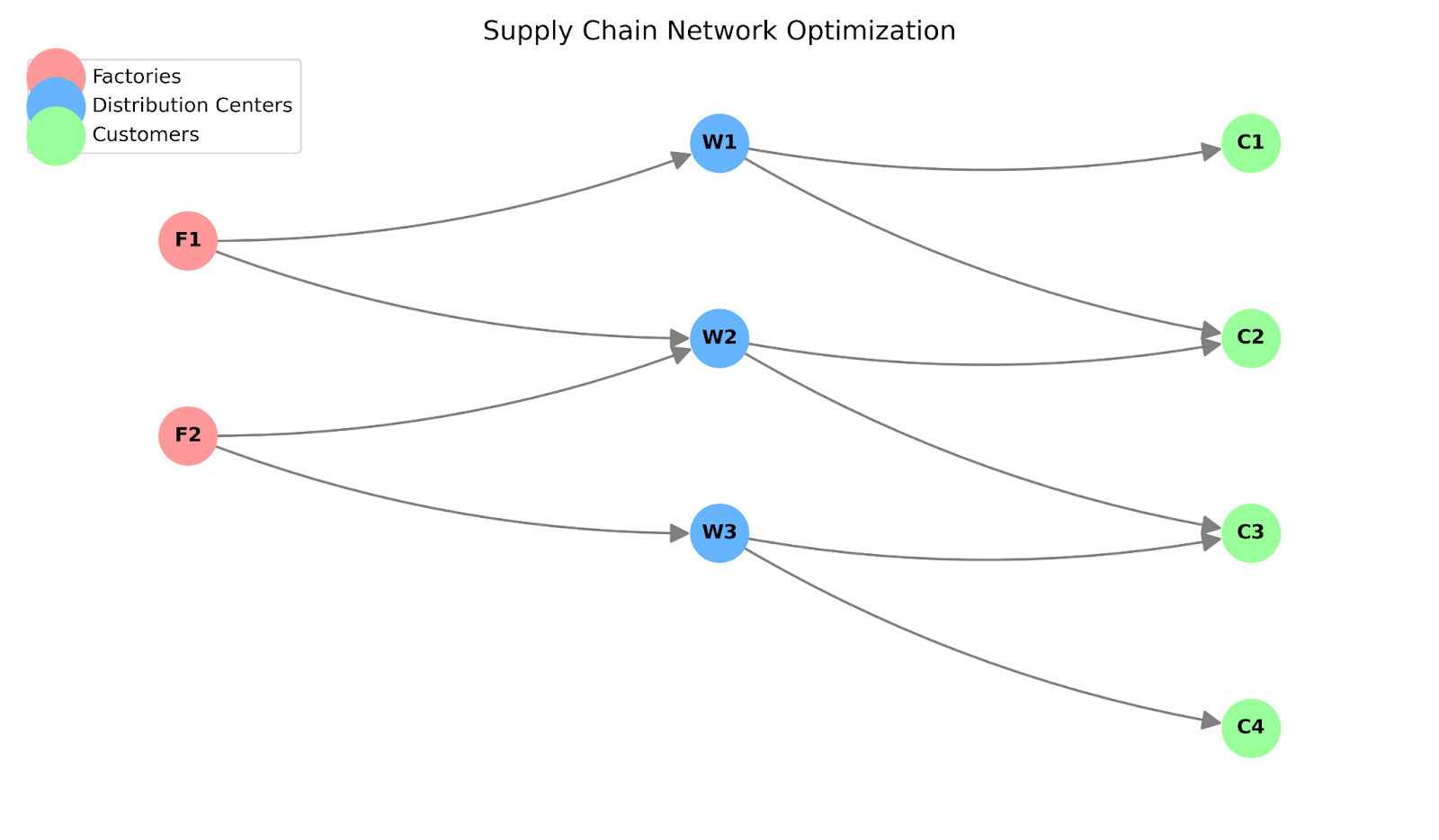
FedEx, UPS, and Amazon use the Supply Chain Analytics in Python course concepts to minimize costs while meeting delivery guarantees.

We will use the Matrix API for this example to handle the scale efficiently.

import gurobipy as gp
from gurobipy import GRB
import numpy as np

# 1. Data Generation
factories = ["F1", "F2"]
warehouses = ["W1", "W2", "W3"]
customers = ["C1", "C2", "C3", "C4"]

# Cost matrices (Factory->Warehouse, Warehouse->Customer)
transport_fw = np.array([[2.0, 4.0, 5.0], [3.0, 1.0, 6.0]])
transport_wc = np.array([
    [1.5, 2.0, 3.0, 4.0],
    [3.0, 1.0, 2.0, 2.5],
    [5.0, 4.0, 1.0, 1.5]
])

# Capacity and Demand
factory_cap = np.array([1000, 1000])
demand = np.array([300, 500, 400, 600])

try:
    with gp.Model("SupplyChain_Matrix") as model:
        # 2. Variables (Matrix Form)
        # Flow F->W and W->C
        flow_fw = model.addMVar((len(factories), len(warehouses)), name="fw")
        flow_wc = model.addMVar((len(warehouses), len(customers)), name="wc")
        
        # Binary decision: Open warehouse?
        open_w = model.addMVar(len(warehouses), vtype=GRB.BINARY, name="open")

        # 3. Objective: Minimize Transport + Fixed Costs
        fixed_cost = 5000
        obj = (transport_fw * flow_fw).sum() + \
              (transport_wc * flow_wc).sum() + \
              (fixed_cost * open_w).sum()
        model.setObjective(obj, GRB.MINIMIZE)

        # 4. Constraints
        # Factory capacity (sum rows of flow_fw <= cap)
        model.addConstr(flow_fw.sum(axis=1) <= factory_cap, name="Cap")

        # Customer demand (sum cols of flow_wc >= demand)
        model.addConstr(flow_wc.sum(axis=0) >= demand, name="Demand")

        # Flow balance: Inflow to W == Outflow from W
        model.addConstr(flow_fw.sum(axis=0) == flow_wc.sum(axis=1), name="Balance")

        # Warehouse capacity linking: Flow out <= BigM * OpenBinary
        model.addConstr(flow_wc.sum(axis=1) <= 2000 * open_w, name="Link")

        model.optimize()

        if model.Status == GRB.OPTIMAL:
            print(f"Optimal Cost: ${model.ObjVal:,.2f}")
            print(f"Open Warehouses: {open_w.X}")

except gp.GurobiError as e:
    print(f"Error: {e}")

This vectorized approach (addMVar, sum(axis=1)) handles thousands of variables instantly, avoiding slow Python loops.

Supply chain network graph. Image by Author.

Inventory optimization

Balancing ordering, holding, and shortage costs is tricky. With uncertain demand, this becomes stochastic optimization, which Gurobi handles via scenario modeling.

Workforce scheduling

Shift planning

Hospitals and call centers must schedule workers while respecting staffing needs, labor rules, and preferences.

This is pure mixed-integer programming. Each assignment is a binary choice. A hospital with 100 nurses and 50 shifts has 5,000 variables to juggle.

Example: nurse scheduling

import gurobipy as gp
from gurobipy import GRB

model = gp.Model("nurse_scheduling")

nurses = ['Alice', 'Bob', 'Carol', 'Dave']
shifts = ['Mon_Day', 'Mon_Night', 'Tue_Day', 'Tue_Night']
min_required = {'Mon_Day': 2, 'Mon_Night': 1, 'Tue_Day': 2, 'Tue_Night': 1}

schedule = model.addVars(nurses, shifts, vtype=GRB.BINARY, name="schedule")

model.setObjective(
    gp.quicksum(schedule[n, s] for n in nurses for s in shifts),
    GRB.MINIMIZE
)

for shift in shifts:
    model.addConstr(
        gp.quicksum(schedule[n, shift] for n in nurses) >= min_required[shift],
        name=f"min_staff_{shift}"
    )

for nurse in nurses:
    model.addConstr(
        gp.quicksum(schedule[nurse, s] for s in shifts) <= 3,
        name=f"max_shifts_{nurse}"
    )

for nurse in nurses:
    # Labor rule: 8-hour rest required between shifts
    model.addConstr(
        schedule[nurse, 'Mon_Day'] + schedule[nurse, 'Mon_Night'] <= 1,
        name=f"no_double_{nurse}_Mon"
    )
    model.addConstr(
        schedule[nurse, 'Tue_Day'] + schedule[nurse, 'Tue_Night'] <= 1,
        name=f"no_double_{nurse}_Tue"
    )

model.optimize()

print("Optimal schedule:")
for nurse in nurses:
    assigned = [s for s in shifts if schedule[nurse, s].X > 0.5]
    print(f"{nurse}: {', '.join(assigned)}")

This models the scheduling problem using binary variables. It minimizes total shifts while respecting staffing needs, maximum hours, and mandatory rest periods.

Financial portfolio optimization

Risk-return trade-off

Portfolio optimization balances expected returns against risk. The classic Markowitz model:

• Maximize: Expected return
• Subject to: Risk (variance) below threshold
• Constraints: Budget constraints, diversification requirements, regulatory limits

This is quadratic programming. Return is linear in portfolio weights, but variance is quadratic (it involves products of weights).

Practical considerations

Real portfolio optimization includes:

• Transaction costs (buying/selling incurs fees)
• Integer constraints (can't buy fractional shares of some assets)
• Regulatory requirements (can't exceed 10% in single security)
• Rebalancing constraints (don't change existing portfolio too drastically)

Asset managers run these optimizations daily, managing billions in capital. Model solve time directly impacts trading strategy execution.

Conclusion

We've covered a lot, from installing Gurobi to building complex supply chain models.

Now, instead of debating opinions in a meeting room, you can put the code on the screen. "Here's the mathematically optimal plan." That changes the conversation. You stop guessing and start proving.

Go ahead and try it on your next messy problem, that scheduling conflict or budget squeeze you've been avoiding. You might just find the perfect answer was hiding in your data all along.

And if you want to sharpen your optimization skills further, check out our Introduction to Linear Programming tutorial and Introduction to Optimization in Python courses to keep building.